Known pulsar analysis pipeline

CWInPy can be used to run an end-to-end pipeline to search for gravitational waves from known pulsars in data from ground-based gravitational-wave detectors. This “known pulsar pipeline” is known here as “knope”.

The pipeline has two main stages:

1. data preprocessing involving heterodyning, filtering and down-sampling raw gravitational-wave detector strain time-series;

2. using the processed data to estimate the posterior probability distributions of the unknown gravitational-wave signal parameter via Bayesian inference.

These stages can be run separately via command line executables, or via their Python APIs, but can be run together using the interface documented here. Comprehensive documentation for the heterodyne and parameter estimation is provided elsewhere on this site and will be required for running the full pipeline.

Running the knope analysis

CWInPy has two command line executables for running knope: cwinpy_knope and cwinpy_knope_pipeline. The former will run the pipeline on the machine on which it is called, while the latter will generate an HTCondor DAG to run the analysis across multiple machines. For example, users of CWInPy within the LVK can run the DAG on collaboration computer clusters. It is also possible to run the analysis via the Open Science Grid if you have access to an appropriate submit machine. In addition to the command line executables, the same results can be using the Python API with the cwinpy.knope.knope() and cwinpy.knope.knope_pipeline() functions, respectively.

It is highly recommended to run this analysis using cwinpy_knope_pipeline (instructions for setting up HTCondor on your own Linux machine are provided here) and the instructions here will focus on that method. A brief description of using cwinpy_knope will be provided, although this should primarily be used, if required, for quick testing.

Note

For LVK users, if requiring access to proprietary IGWN frame data (i.e., non-public frames visible to those within the LVK collaboration) via CVMFS rather than frames locally stored on a cluster, you will need to generate a SciToken to allow the analysis script to access them. To enable the pipeline script to find science segments and frame URLs you must generate a token with:

htgettoken -a vault.ligo.org -i igwn

Warning

On some systems still using the X.509 authentication you may instead need to run

ligo-proxy-init -p albert.einstein

to find the science segments and frame URLs.

and then run:

condor_vault_storer -v igwn

to allow the HTCondor jobs to access the credentials.

In many of the examples below we will assume that you are able to access the open LIGO and Virgo data available from the GWOSC via CVMFS. To find out more about accessing this data see the instructions here.

Configuration file

The primary way to run the pipeline is by supplying the cwinpy_knope_pipeline executable with a configuration file. This configuration file will be a concatenation of the configurations that are separately required for the data processing using cwinpy_heterodyne_pipeline and the parameter estimation using cwinpy_pe_pipeline. You should consult those parts of the documentation for more detail on the input parameters in each case.

Note

In the case of the cwinpy_knope_pipeline configuration, the inputs to the parameter estimation stage (pulsar parameter files and heterodyned data files) will be set automatically from the outputs of the data processing stage.

Any parameters used for simulated data in the parameter estimation [pe] part will also be ignored.

An example configuration file, with inline comments describing the inputs, is given below:

[run]
# the base directory for the analysis **output**
basedir = /home/username/analysis

######### Condor DAG specific inputs ########
[heterodyne_dag]
# the location of the directory to contain the Condor DAG submission files
# (defaults to "basedir/submit")
;submit = 

# a flag specifying whether to automatically submit the DAG after its creation
# (defaults to False)
submitdag = False

# a flag saying whether to build the DAG (defaults to True)
;build =

# set whether running on the OSG (defaults to False). If using the OSG it
# expects you to be within an IGWN conda environment or using the singularity
# container option below.
;osg =

# if wanting to run on the OSG with the latest development version of cwinpy,
# which is within a Singularity container, set this flag to True
;singularity

# set whether Condor should transfer files to/from the local run node (default
# is True). Note that if using "transfer_files" (or OSG above) all input files,
# e.g., pulsar parameter files, input frame cache files or segment files, or
# inputs of previously heterodyned data files, should have unique file names as
# when they are transferred there will be a flat directory structure.
;transfer_files =

# if running on the OSG you can select desired sites to run on
# see https://computing.docs.ligo.org/guide/condor/submission/#DESIRED_Sites
;desired_sites =
;undesired_sites =

######## cwinpy_heterodyne Job options ########
[heterodyne_job]
# the location of the cwinpy_heterodyne executable to use (defaults to try and
# find cwinpy_heterodyne in the current user PATH)
;executable =

# set the Condor universe (defaults to "vanilla") 
;universe =

# directory location for the output from stdout from the Job (defaults to
# "basedir/out")
;out =

# directory location for the output from stderr from the Job (defaults to
# "basedir/error")
;error =

# directory location for any logging information from the jobs (defaults to
# "basedir/log")
;log =

# the location of the directory to contain the Condor job submission files
# (defaults to "basedir/submit")
;submit =

# set to allow the jobs to access local environment variables (defaults to
# True)
getenv = True

# the amount of available memory request for each job (defaults to 16 Gb)
# [Note: this is required for vanilla jobs on LIGO Scientific Collaboration
# computer clusters]
;request_memory =

# the amount of disk space required for each job (defaults to 2 Gb)
# [Note: this is required for vanilla jobs on LIGO Scientific Collaboration
# computer clusters]
;request_disk =

# the number of CPUs the job requires (defaults to 1, cwinpy_heterodyne is not
# currently parallelised in any way)
;request_cpus =

# additional Condor job requirements (defaults to None)
;requirements =

# set how many times the DAG will retry a job on failure (default to 2)
;retry =

# Job accounting group and user [Note: these are required on LIGO Scientific
# Collaboration computer clusters, but may otherwise be left out, see
# https://accounting.ligo.org/user for details of valid accounting tags
;accounting_group =
accounting_group_user = albert.einstein

[ephemerides]
# This specifies the pulsar parameter files for which to heterodyne the data.
# It can be either:
# - a string giving the path to an individual pulsar TEMPO(2)-style parameter
#   file
# - a string giving the path to a directory containing multiple TEMPO(2)-style
#   parameter files (the path will be recursively searched for any file with
#   the extension ".par")
# - a list of paths to individual pulsar parameter files
# - a dictionary containing paths to individual pulsars parameter files keyed
#   to their names.
# If instead, pulsar names are given rather than parameter files it will
# attempt to extract an ephemeris for those pulsars from the ATNF pulsar
# catalogue. If such ephemerides are available then they will be used
# (notification will be given when this is these cases).
pulsarfiles = /home/username/pulsars

# You can analyse only particular pulsars from those specified by parameter
# files found through the "pulsarfiles" argument by passing a string, or list
# of strings, with particular pulsars names to use.
;pulsars =

# Locations of the Earth and Sun ephemerides. If not given then the ephemerides
# will be automatically determined from the pulsar parameter information. The
# values should be dictionaries keyed to the ephemeris type, e.g., "DE405", and
# pointing to the location of the ephemeris file.
;earth =
;sun =

######## heterodyne specific options ########
[heterodyne]
# A list of the prefix names of the set of gravitational wave detectors to use.
# If only one detector is being used it does not need to be given as a list.
detectors = ["H1", "L1"]

# A list, or single value, with the frequency scale factors at which to
# heterodyne the data. By default this will have a value of 2, i.e., heterodyne
# at twice the pulsar's rotation frequency
;freqfactors =

# A dictionary containing the start times of the data to use for each detector.
# These start times can be lists if multiple different datasets are being used,
# e.g., O1 and O2, where different channel names or DQ flags might be required.
# If a single value is given it is used for all detectors.
starttimes = {"H1": [1125969918, 1164556817], "L1": [1126031358, 1164556817]}

# A dictionary containing the end times of the data to use for each detector.
# These end times can be lists if multiple different datasets are being used,
# e.g., O1 and O2, where different channel names or DQ flags might be required.
# If a single value is given it is used for all detectors.
endtimes = {"H1": [1137258494, 1187733618], "L1": [1137258494, 1187733618]}

# The length of time in integer seconds to "stride" through the data, i.e.,
# read-in and heterodyne in one go. Default is 3600 seconds.
;stride =

# The (on average) length of data (in seconds) for which to split into
# individual (coarse or one-stage) heterodyning jobs for a particular detector
# and frequency factor. Default is 86400, i.e., use a days worth data for each
# job. If wanting to just have a single job for all data then set this to 0.
joblength = 86400

# The number of jobs over which to split up the (coarse or one-stage)
# heterodyning over pulsars for a particular detector and frequency factor.
# Default is 1. Use this to prevent too many files being required to be
# transferred if running over the OSG.
;npulsarjobs =

# The frame "types" to search for containing the required strain data. This
# should be a dictionary, keyed to detector names (with the same names as in
# the detectors list and starttimes/endtimes dictionaries). For each detector
# there should be a single frame type, or if multiple start times and end times
# are given there should be a list of frame types for each time segment (i.e., 
# different frame types for different observing runs). Alternatively, frame
# cache files (or lists of frame cache files for different time spans) can be
# provided using the framecache value below, which contain pre-made lists of
# frame files.
frametypes = {"H1": ["H1_HOFT_C02", "H1_CLEANED_HOFT_C02"], "L1": ["L1_HOFT_C02", "L1_CLEANED_HOFT_C02"]}

# If you have a pre-generated cache of frame files for each detector, or the
# path to a directory that contains frames files (they can be found recursively
# within sub-directories of the supplied directory), they can be supplied
# instead of (or with, if suppling a directory) the frametypes option. This
# should be in the form of a dictionary and keyed to the detector names. If
# there are multiple start times each dictionary item can be a list containing
# a file for that given time segment.
;framecaches =

# This specficies the channels with the gravitational-wave frame files from
# which to extract the strain data. This should be in the form of a dictionary
# and keyed to the detector names. If there are multiple start times each
# dictionary item can be a list containing the channel for that given time
# segment. 
channels = {"H1": ["H1:DCS-CALIB_STRAIN_C02", "H1:DCH-CLEAN_STRAIN_C02"], "L1": ["L1:DCS-CALIB_STRAIN_C02", "L1:DCH-CLEAN_STRAIN_C02"]}

# This specifies whether to strictly require that all frame files that are
# requested are able to be read in, otherwise an exception is raised. This
# defaults to False, allowing corrupt/missing frame files to be ignored.
;strictdatarequirement =

# This specifies the server name used to find the frame information if
# using the frametypes option. E.g., use https://gwosc.org for
# open data direct from GWOSC, or datafind.gwosc.org for open data via
# CVMFS. LVK collaboration members can use datafind.ligo.org:443 to find data.
host = datafind.ligo.org:443

# This specifies the server name used to find data quality segment information.
# By default this will use the server https://segments.ligo.org if nothing is
# given and the segmentlist option below is not used.
;segmentserver =

# If querying the segment server the date segment to use are specified by the
# flags that you want to include. This should be a dictionary, keyed to the
# detector name (with the same names as in the detectors list and
# starttimes/endtimes dictionaries). For each detector there should be a single
# data quality flag name, or if multiple start and end times are given there
# should be a list of data quality flags for each segment.
includeflags = {"H1": ["H1:DCS-ANALYSIS_READY_C02", "H1:DCH-CLEAN_SCIENCE_C02:1"], "L1": ["L1:DCS-ANALYSIS_READY_C02", "L1:DCH-CLEAN_SCIENCE_C02:1"]}

# Data quality segments to exclude from analysis can also be set. This should
# be a dictionary keyed to the detector names. For each detector multiple
# exclusion flags can be used. If there are multiple start and end times the
# exclusion flags for each segment should be given in a list, and within the
# list multiple flags for the same segment should be separated by commas. If no
# exclusions are required for a given segment then an empty string should be
# given.
excludeflags = {"H1": ["H1:DCS-BAD_STRAIN_H1_HOFT_C02:1,H1:DCS-BAD_KAPPA_BASIC_CUT_H1_HOFT_C02:1", ""], "L1": ["L1:DCS-BAD_KAPPA_BASIC_CUT_L1_HOFT_C02:1", ""]}

# Rather than having the pipeline produce the segment lists, pre-generated
# segment list files can be passed to the code. This should be given as a
# dictionary keyed to the detector names. For each detector a file containing
# the segments (plain ascii text with two columns giving the start and end of
# each segment) should be given, or for multiple start and end times, lists of
# files can be given.
;segmentlists =

# Set whether the heterodyne in performed in one stage (set to 1) or two
# stages, the so-called "coarse" and "fine" heterodyne (set to 2). Default is
# to use one stage.
;stages =

# The rate at which to resample the data. If performing the heterodyne in one
# stage this should be a single value, if performing it in two stages it should
# be a list with the first value being the resample rate for the first stage
# and the second being the resample rate for the second stage. By default, the
# final sample rate in either case is 1/60 Hz, and for a two stage process the
# first resample rate of 1 Hz.
;resamplerate =

# The knee frequency (Hz) of the low-pass filter applied after heterodyning the
# data. This should only be given when heterodying raw strain data and not if
# re-heterodyning processed data. Default is 0.1 Hz is heterodyning in one
# stage and 0.5 Hz if heterodyning over two stages.
;filterknee =

# The order of the low-pass Butterworth filter applied after heterodyning the
# data. The default is 9.
;filterorder =

# The number of seconds to crop from the start and end of data segments after
# the initial heterodyned to remove filter impulse effects and issues prior to
# lock-loss. Default is 60 seconds.
;crop =

# The location of previously heterodyned data files for input. This should be a
# string or dictionary of strings containing the full file path, or directory
# path, pointing the the location of pre-heterodyned data. For a single pulsar
# a file path can be given. For multiple pulsars a directory containing
# heterodyned files (in HDF5 or txt format) can be given provided that within
# it the file names contain the pulsar names as supplied in the file input with
# pulsarfiles. Alternatively, a dictionary can be supplied, keyed on the pulsar
# name, containing a single file path, a directory path as above, or a list of
# files/directories for that pulsar. If supplying a directory, it can contain
# multiple heterodyned files for a each pulsar and all will be used. 
;heterodyneddata = 

# The directory location to output the heterodyned data files. If performing
# the heterodyne in one stage this should be a single string containing the
# name of the directory to output data to (which will be created if it does not
# exist), or a dictionary keyed by detector name pointing to output directories
# for each detector. If performing the heterodyne in two stages this should be
# a list containing two items, each of which would be consistent with the above
# information.
outputdir = {"H1": "/home/username/analysis/heterodyne/H1", "L1": "/home/username/analysis/heterodyne/L1"}

# A label used for the output filename. If performing the heterodyne in one
# stage this can be a single value, or for two stages can be a list with an
# item for the value to use for each stage. By default the label naming
# convention follows:
# heterodyne_{psr}_{det}_{freqfactor}_{gpsstart}-{gpsend}.hdf5
# where the keys are used to based on the analysis values. These keys can be
# used in alternative labels.
;label =

# A flag to set whether to correct the signal to the solar system barycentre.
# For a one stage heterodyne this should just be a boolean value (defaulting to
# True). For a two stage heterodyne it should be a list containing a boolean
# value for the coarse stage and the fine stage (defaulting to [False, True]).
includessb = True

# A flag to set whether to correct the signal to the binary system barycentre
# if required. See includessb for the format and defaults.
includebsb = True

# A flag to set whether to correct the signal for any glitch induced phase
# evolution if required. See includessb for the format and defaults.
includeglitch = True

# A flag to set whether to correct the signal for any sinusoidal WAVES
# parameters used to model timing noise if required. See includessb for the
# format and defaults.
includefitwaves = True

# The pulsar timing package TEMPO2 can be used to calculate the pulsar phase
# evolution rather than the LAL functions. To do this set the flag to True.
# TEMPO2 and the libstempo package must be installed. This can only be used if
# performing the heterodyne as a single stage. The solar system ephemeris files
# and include... flags will be ignored. All components of the signal model
# (e.g., binary motion or glitches) will be included in the phase generation.
;usetempo2 =

# If performing the full heterodyne in one step it is quicker to interpolate
# the solar system barycentre time delay and binary barycentre time delay. This
# sets the step size, in seconds, between the points in these calculations that
# will be the interpolation nodes. The default is 60 seconds.
;interpolationstep =

# Set this flag to make sure any previously generated heterodyned files are
# overwritten. By default the analysis will "resume" from where it left off,
# such as after forced Condor eviction for checkpointing purposes. Therefore,
# this flag is needs to be explicitly set to True (the default is False) if
# not wanting to use resume.
;overwrite =

######## options for merging heterodyned files ########
[merge]
# Merge multiple heterodyned files into one. The default is True
;merge =

# Overwrite existing merged file. The default is True
;overwrite =

# Remove inidividual pre-merged files. The default is False.
remove = True

######### Condor DAG specific inputs ########
[pe_dag]
# the location of the directory to contain the Condor DAG submission files
# (defaults to "basedir/submit")
;submit = 

# a flag specifying whether to automatically submit the DAG after its creation
# (defaults to False)
submitdag = False

# a flag saying whether to build the DAG (defaults to True)
;build =

# any additional submittion options (defaults to None)
;submit_options =

# the scheduler (Condor or Slurm) to use (defaults to Condor)
;scheduler

######## cwinpy_pe Job options ########
[pe_job]
# the location of the cwinpy_pe executable to use (defaults to try and find
# cwinpy_pe in the current user PATH)
;executable =

# the prefix of the name for the Condor Job submit file (defaults to
# "cwinpy_pe")
;name =

# set the Condor universe (defaults to "vanilla") 
;universe =

# directory location for the output from stdout from the Job (defaults to
# "basedir/out")
;out =

# directory location for the output from stderr from the Job (defaults to
# "basedir/error")
;error =

# directory location for any logging information from the jobs (defaults to
# "basedir/log")
;log =

# the location of the directory to contain the Condor job submission files
# (defaults to "basedir/submit")
;submit =

# the amount of available memory request for each job (defaults to 4 Gb)
# [Note: this is required for vanilla jobs on LIGO Scientific Collaboration
# computer clusters]
;request_memory =

# the amount of disk space required for each job (defaults to 1 Gb)
# [Note: this is required for vanilla jobs on LIGO Scientific Collaboration
# computer clusters]
;request_disk =

# the number of CPUs the job requires (defaults to 1, cwinpy_pe is not
# currently parallelised in any way)
;request_cpus =

# additional Condor job requirements (defaults to None)
;requirements =

# set how many times the DAG will retry a job on failure (default to 2)
;retry =

# Job accounting group and user [Note: these are required on LIGO Scientific
# Collaboration computer cluster, but may otherwise be left out, see
; https://accounting.ligo.org/user for valid accounting tags]
;accounting_group =
accounting_group_user = albert.einstein

######## PE specific options ########
[pe]

# The number of parallel runs for each pulsar. These will be combined to
# create the final output. This defaults to 1.
;n_parallel =

# The period for automatically restarting HTCondor PE jobs to prevent a hard
# eviction. If not given this defaults to 43200 seconds
;periodic-restart-time =

# The directory within basedir into which to output the results in individual
# directories named using the PSRJ name (defaults to "results")
;results =

# Pulsar "injection" parameter files containing simulated signal parameters to
# add to the data. If not given then no injections will be performed. If given
# it should be in the same style as the "pulsars" section.
;injections =

# Set this boolean flag to state whether to run parameter estimation with a
# likelihood that uses the coherent combination of data from all detectors
# specified. This defaults to True.
;coherent =

# Set this boolean flag to state whether to run the parameter estimation for
# each detector independently. This defaults to False.
;incoherent =

# Set a dictionary of keyword arguments to be used by the HeterodynedData class
# that the data files will be read into.
;data_kwargs = {}

# The prior distributions to use for each pulsar. The value of this can either
# be:
#  - a single prior file (in bilby format) to use for all pulsars
#  - a list of prior files, where each filename contains the PSRJ name of the
#    associated pulsar
#  - a directory, or glob-able directory pattern, containing the prior files,
#    where each filename contains the PSRJ name of the associated pulsar
#  - a dictionary with prior file names keyed to the associated pulsar
# If not given then default priors will be used. If using data at just twice
# the rotation frequency the default priors are:
#   h0 = Uniform(minimum=0.0, maximum=1.0e-22, name='h0')
#   phi0 = Uniform(minimum=0.0, maximum=pi, name='phi0')
#   iota = Sine(minimum=0.0, maximum=pi, name='iota')
#   psi = Uniform(minimum=0.0, maximum=pi/2, name='psi')
# For data at just the rotation frequency the default priors are:
#   c21 = Uniform(minimum=0.0, maximum=1.0e-22, name='c21')
#   phi21 = Uniform(minimum=0.0, maximum=2*pi, name='phi21')
#   iota = Sine(minimum=0.0, maximum=pi, name='iota')
#   psi = Uniform(minimum=0.0, maximum=pi/2, name='psi')
# And, for data at both frequencies, the default priors are:
#   c21 = Uniform(minimum=0.0, maximum=1.0e-22, name='c21')
#   c22 = Uniform(minimum=0.0, maximum=1.0e-22, name='c22')
#   phi21 = Uniform(minimum=0.0, maximum=2*pi, name='phi21')
#   phi22 = Uniform(minimum=0.0, maximum=2*pi, name='phi22')
#   iota = Sine(minimum=0.0, maximum=pi, name='iota')
#   psi = Uniform(minimum=0.0, maximum=pi/2, name='psi')
priors = /home/username/analysis/priors

# Flag to say whether to output the injected/recovered signal-to-noise ratios
# (defaults to False)
;output_snr =

# The location within basedir for the cwinpy_pe configuration files
# generated to each source (defaults to "configs")
;config =

# The stochastic sampling package to use (defaults to "dynesty")
;sampler =

# A dictionary of any keyword arguments required by the sampler package
# (defaults to None)
;sampler_kwargs =

# A flag to set whether to use the numba-enable likelihood function (defaults
# to True)
;numba =

# A flag to set whether to generate and use a reduced order quadrature for the
# likelihood calculation (defaults to False)
;roq =

# A dictionary of any keyword arguments required by the ROQ generation
;roq_kwargs =

Quick setup

The cwinpy_knope_pipeline script has some quick setup options that allow an analysis to be launched in one line without the need to define a configuration file. These options require that the machine/cluster that you are running HTCondor on has access to open data from GWOSC available via CVMFS. It is also recommended that you run CWInPy from within an IGWN conda environment

For example, if you have a TEMPO(2)-style pulsar parameter file, e.g., J0740+6620.par, and you want to analyse the open O1 data for the two LIGO detectors you can simply run:

cwinpy_knope_pipeline --run O1 --pulsar J0740+6620.par --output /home/usr/O1

where /home/usr/O1 is the name of the directory where the run information and results will be stored (if you don’t specify an --output then the current working directory will be used). This command will automatically submit the HTCondor DAG for the job. To specify multiple pulsars you can use the --pulsar option multiple times. If you do not have a parameter file for a pulsar you can instead use the ephemeris given by the ATNF pulsar catalogue. To do this you need to instead supply a pulsar name (as recognised by the catalogue), for example, to run the analysis using O2 data for the pulsar J0737-3039A you could do:

cwinpy_knope_pipeline --run O2 --pulsar J0737-3039A --output /home/usr/O2

Internally the ephemeris information is obtained using the QueryATNF class from psrqpy.

Note

Any pulsar parameter files extracted from the ATNF pulsar catalogue will be held in a subdirectory of the directory from which you invoked the cwinpy_knope_pipeline script, called atnf_pulsars. If such a directory already exists and contains the parameter file for a requested pulsar, then that file will be used rather than being reacquired from the catalogue. To ensure files are up-to-date, clear out the atnf_pulsars directory as required.

CWInPy also contains information on the continuous hardware injections performed in each run, so if you wanted the analyse the these in, say, the LIGO sixth science run, you could do:

cwinpy_knope_pipeline --run S6 --hwinj --output /home/usr/hwinjections

Other command line arguments for cwinpy_knope_pipeline, e.g., for setting specific detectors, can be found below. If running on a LIGO Scientific Collaboration cluster the --accounting-group flag must be set to a valid accounting tag, e.g.,:

cwinpy_knope_pipeline --run O1 --hwinj --output /home/user/O1injections --accounting-group ligo.prod.o1.cw.targeted.bayesian

Note

The quick setup will only be able to use default parameter values for the heterodyne and parameter estimation. For “production” analyses, or if you want more control over the parameters, it is recommended that you use a configuration file to set up the run.

The frame data used by the quick setup defaults to that with a 4096 Hz sample rate. However, if analysing sources with frequencies above about 1.6 kHz this should be switched, using the --samplerate flag to using the 16 kHz sampled data. By default, if analysing hardware injections for any of the advanced detector runs the 16 kHz data will be used due to frequency of the fastest pulsar being above 1.6 kHz.

knope examples

A selection of example configuration files for using with cwinpy_knope_pipeline are shown below. These examples are generally fairly minimal and make use of many default settings. If basing your own configuration files on these, the various input and output directory paths should be changed. These all assume a user matthew.pitkin running on the ARCCA Hawk Computing Centre or the LDAS@Caltech cluster.

Note

When running an analysis it is always worth regularly checking on the Condor jobs using condor_q. There is no guarantee that all jobs will successfully complete or that some jobs might not get held for some reason. These may require some manual intervention such as resubmitting a generated rescue DAG or releasing held jobs after diagnosing and fixing (maybe via condor_qedit) the hold reason.

O1 LIGO (proprietary) data, single pulsar

An example configuration file for performing a search for a single pulsar, the Crab pulsar (J0534+2200), for a signal emitted from the \(l=m=2\) harmonic, using proprietary O1 LIGO data can be downloaded here and is reproduced below:

[run]
basedir = /home/matthew.pitkin/projects/cwinpyO1

[knope_job]
accounting_group = ligo.prod.o1.cw.targeted.bayesian
accounting_group_user = matthew.pitkin

[ephemerides]
pulsarfiles = /home/matthew.pitkin/projects/O1pulsars
pulsars = J0534+2200

[heterodyne]
detectors = ["H1", "L1"]
freqfactors = 2
starttimes = 1126051217
endtimes = 1137254417
frametypes = {"H1": "H1_HOFT_C02", "L1": "L1_HOFT_C02"}
channels = {"H1": "H1:DCS-CALIB_STRAIN_C02", "L1": "L1:DCS-CALIB_STRAIN_C02"}
host = datafind.ligo.org:443
includeflags = {"H1": "H1:DCS-ANALYSIS_READY_C02", "L1": "L1:DCS-ANALYSIS_READY_C02"}
excludeflags = {"H1": "H1:DCS-BAD_STRAIN_H1_HOFT_C02:1,H1:DCS-BAD_KAPPA_BASIC_CUT_H1_HOFT_C02:1", "L1": "L1:DCS-BAD_KAPPA_BASIC_CUT_L1_HOFT_C02:1"}
outputdir = {"H1": "/home/matthew.pitkin/projects/cwinpyO1/heterodyne/H1", "L1": "/home/matthew.pitkin/projects/cwinpyO1/heterodyne/L1"}

[merge]
remove = True

[pe_dag]
submitdag = True

[pe]
priors = /home/matthew.pitkin/projects/O1priors

This requires a pulsar parameter file for the Crab pulsar within the /home/matthew.pitkin/projects/O1pulsars directory and a prior file, called e.g., J0534+2200.prior in the /home/matthew.pitkin/projects/O1priors directory. An example prior file might contain:

h0 = FermiDirac(1.0e-24, mu=1.0e-22, name='h0')
phi0 = Uniform(minimum=0.0, maximum=pi, name='phi0')
iota = Sine(minimum=0.0, maximum=pi, name='iota')
psi = Uniform(minimum=0.0, maximum=pi/2, name='psi')

This would be run with:

$ cwinpy_knope_pipeline knope_example_O1_ligo.ini

Note

Before running this (provided you have installed the SciTokens tools) you should run:

$ htgettoken --audience https://datafind.ligo.org --scope gwdatafind.read -a vault.ligo.org --issuer igwn

to generate SciTokens authentication for accessing the proprietary data via CVMFS.

Once complete, this example should have generated the heterodyned data files for H1 and L1 (within the /home/matthew.pitkin/projects/cwinpyO1/heterodyne directory):

from cwinpy import MultiHeterodynedData

het = MultiHeterodynedData(
   {
       "H1": "H1/heterodyne_J0534+2200_H1_2_1126073529-1137253524.hdf5",
       "L1": "L1/heterodyne_J0534+2200_L1_2_1126072156-1137250767.hdf5",
   }
)

fig = het.plot(together=True, remove_outliers=True)
fig.show()

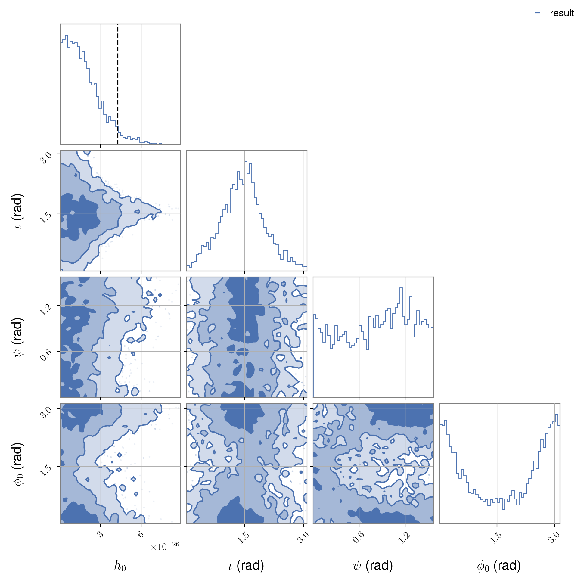
and the posterior samples for an analysis using both LIGO detectors (within the /home/matthew.pitkin/projects/cwinpyO1/results directory):

from cwinpy.plot import Plot

plot = Plot(
   "J0534+2200/cwinpy_pe_H1L1_J0534+2200_result.hdf5",
   parameters=["h0", "iota", "psi", "phi0"].
)
plot.plot()

# add 95% upper limit line
plot.fig.get_axes()[0].axvline(
   plot.upper_limit(parameter="h0"),
   color="k",
   ls="--",
)

plot.fig.show()

Note

To run the example and also perform parameter estimation for each individual detector (rather than just the coherent multi-detector analysis), the additional option incoherent = True should be added in the [pe] section of the configuration file.

O1 & O2 LIGO/Virgo (open) data, multiple pulsars

An example configuration file for performing a search for multiple pulsars, for a signal emitted from the \(l=m=2\) harmonic, using open O1 and O2 LIGO and Virgo data can be downloaded here and is reproduced below:

[run]
basedir = /home/matthew.pitkin/projects/cwinpyO2

[knope_job]
accounting_group = ligo.prod.o2.cw.targeted.bayesian
accounting_group_user = matthew.pitkin

[ephemerides]
pulsarfiles = /home/matthew.pitkin/projects/O2pulsars

[heterodyne]
detectors = ["H1", "L1", "V1"]
freqfactors = 2
starttimes = {"H1": [1126051217, 1164556817], "L1": [1126051217, 1164556817], "V1": [1185624018]}
endtimes = {"H1": [1137254417, 1187733618], "L1": [1137254417, 1187733618], "V1": [1187733618]}
frametypes = {"H1": ["H1_LOSC_4_V1", "H1_GWOSC_O2_4KHZ_R1"], "L1": ["L1_LOSC_4_V1", "L1_GWOSC_O2_4KHZ_R1"], "V1": ["V1_GWOSC_O2_4KHZ_R1"]}
channels = {"H1": ["H1:LOSC-STRAIN", "H1:GWOSC-4KHZ_R1_STRAIN"], "L1": ["L1:LOSC-STRAIN", "L1:GWOSC-4KHZ_R1_STRAIN"], "V1": ["V1:GWOSC-4KHZ_R1_STRAIN"]}
host = datafind.gwosc.org
includeflags = {"H1": ["H1_CBC_CAT1", "H1_CBC_CAT1"], "L1": ["L1_CBC_CAT1", "L1_CBC_CAT1"], "V1": ["V1_CBC_CAT1"]}
outputdir = {"H1": "/home/matthew.pitkin/projects/cwinpyO2/heterodyne/H1", "L1": "/home/matthew.pitkin/projects/cwinpyO2/heterodyne/L1", "V1": "/home/matthew.pitkin/projects/cwinpyO2/heterodyne/V1"}
usetempo2 = True

[merge]
remove = True

[pe_dag]
submitdag = True

[pe]
priors = /home/matthew.pitkin/projects/O2priors/priors.txt
incoherent = True

This requires the parameter files for the pulsars to be within the /home/matthew.pitkin/projects/O2pulsars directory (in the example results shown below this directory contained files for the two pulsars J0737-3039A and J1843-1113). In this example, a single prior file for all pulsars is used at the location /home/matthew.pitkin/projects/O2priors/priors.txt directory. This might contain, e.g.,

h0 = FermiDirac(1.0e-24, mu=1.0e-22, name='h0')
phi0 = Uniform(minimum=0.0, maximum=pi, name='phi0')
iota = Sine(minimum=0.0, maximum=pi, name='iota')
psi = Uniform(minimum=0.0, maximum=pi/2, name='psi')

Due to using data from two runs, the start and end times of each run need to be specified (the lists within the associated dictionaries), and appropriate frame types, channels and segment types need to be provided for each run.

In this example, it uses TEMPO2 (via libstempo) for calculating the phase evolution of the signal. Due to the incoherent = True value in the [pe] section, this analysis will perform parameter estimation for each pulsar for each individual detector and also for the full multi-detector data set.

This would be run with:

$ cwinpy_knope_pipeline knope_example_O2_open.ini

Displaying the results

Once the analysis is complete, a table of upper limits can be produced using the UpperLimitTable class (this requires the cweqgen package to be installed as it makes used of the cweqgen.equations.equations() function). The UpperLimitTable class is a child of an astropy.table.QTable and retains all its attributes. We can, for example, create a table showing the 95% upper limits on amplitude, ellipticity, mass quadrupole and the ratio to the spin-down limits:

from cwinpy.pe import UpperLimitTable

# directory containing the parameter estimation results
resdir = "/home/matthew.pitkin/projects/cwinpyO2/results"

tab = UpperLimitTable(
    resdir=resdir,
    ampparam="h0",  # get the limits on h0
    includeell=True,  # calculate the ellipticity limit
    includeq22=True,  # calculate the mass quadrupole limit
    includesdlim=True,  # calculate the spin-down limit and ratio
    upperlimit=0.95,  # calculate the 95% credible upper limit (the default)
)

# output the table in rst format, so it renders nicely in these docs!
print(tab.table_string(format="rst"))

PSRJ	F0ROT	F1ROT	DIST	H0_L1_95%UL	ELL_L1_95%UL	Q22_L1_95%UL	SDRAT_L1_95%UL	SDLIM	H0_H1L1V1_95%UL	ELL_H1L1V1_95%UL	Q22_H1L1V1_95%UL	SDRAT_H1L1V1_95%UL	H0_H1_95%UL	ELL_H1_95%UL	Q22_H1_95%UL	SDRAT_H1_95%UL	H0_V1_95%UL	ELL_V1_95%UL	Q22_V1_95%UL	SDRAT_V1_95%UL
J0737-3039A	44.05	-3.41×10-15	1.10	2.52×10-26	3.37×10-6	2.61×1032	3.9	6.45×10-27	1.59×10-26	2.13×10-6	1.64×1032	2.46	1.84×10-26	2.47×10-6	1.91×1032	2.85	1.65×10-25	2.21×10-5	1.71×1033	25
J1843-1113	541.81	-2.78×10-15	1.26	7.53×10-26	7.64×10-8	5.9×1030	51	1.45×10-27	4.52×10-26	4.59×10-8	3.54×1030	31	1.03×10-25	1.05×10-7	8.1×1030	71	9.91×10-25	1.01×10-6	7.77×1031	683

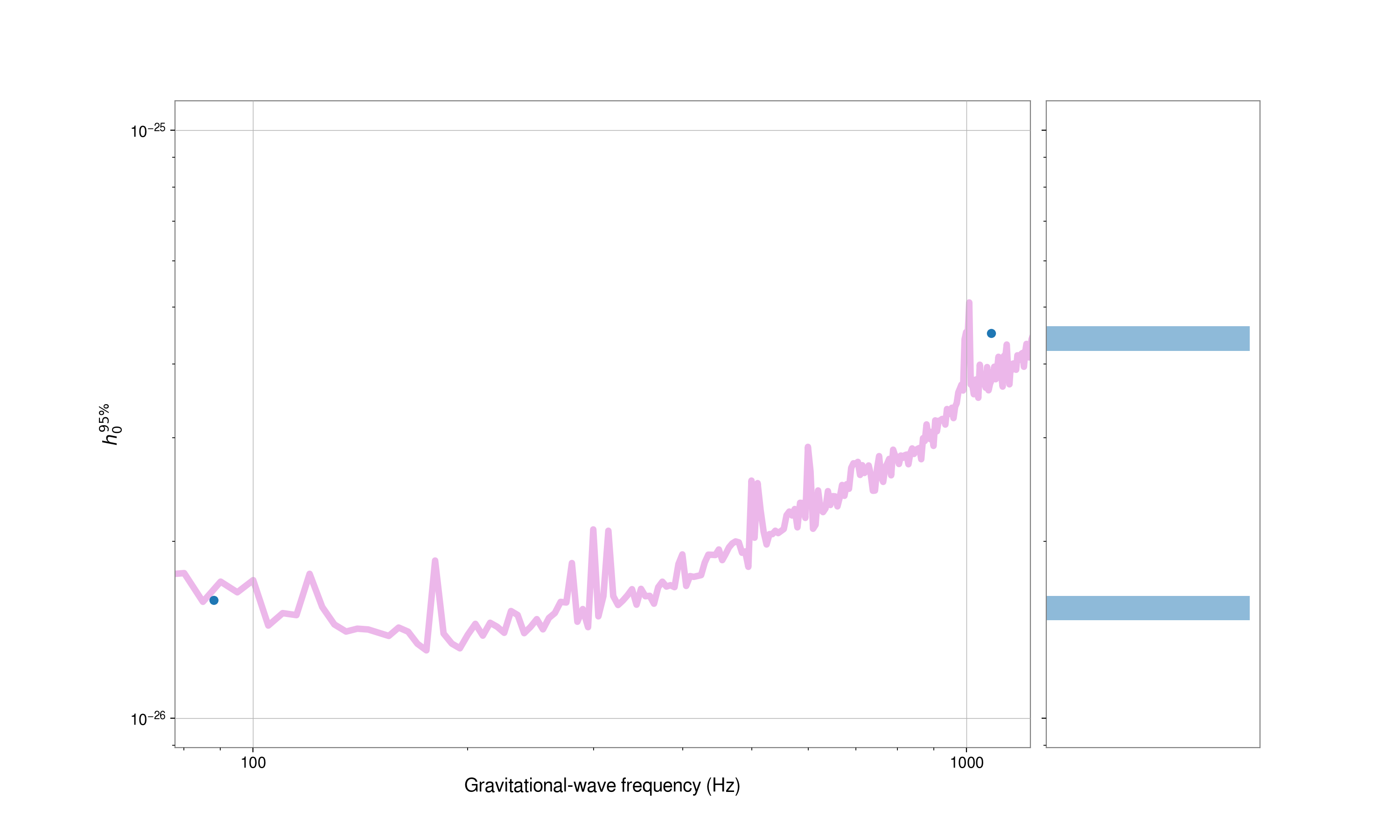
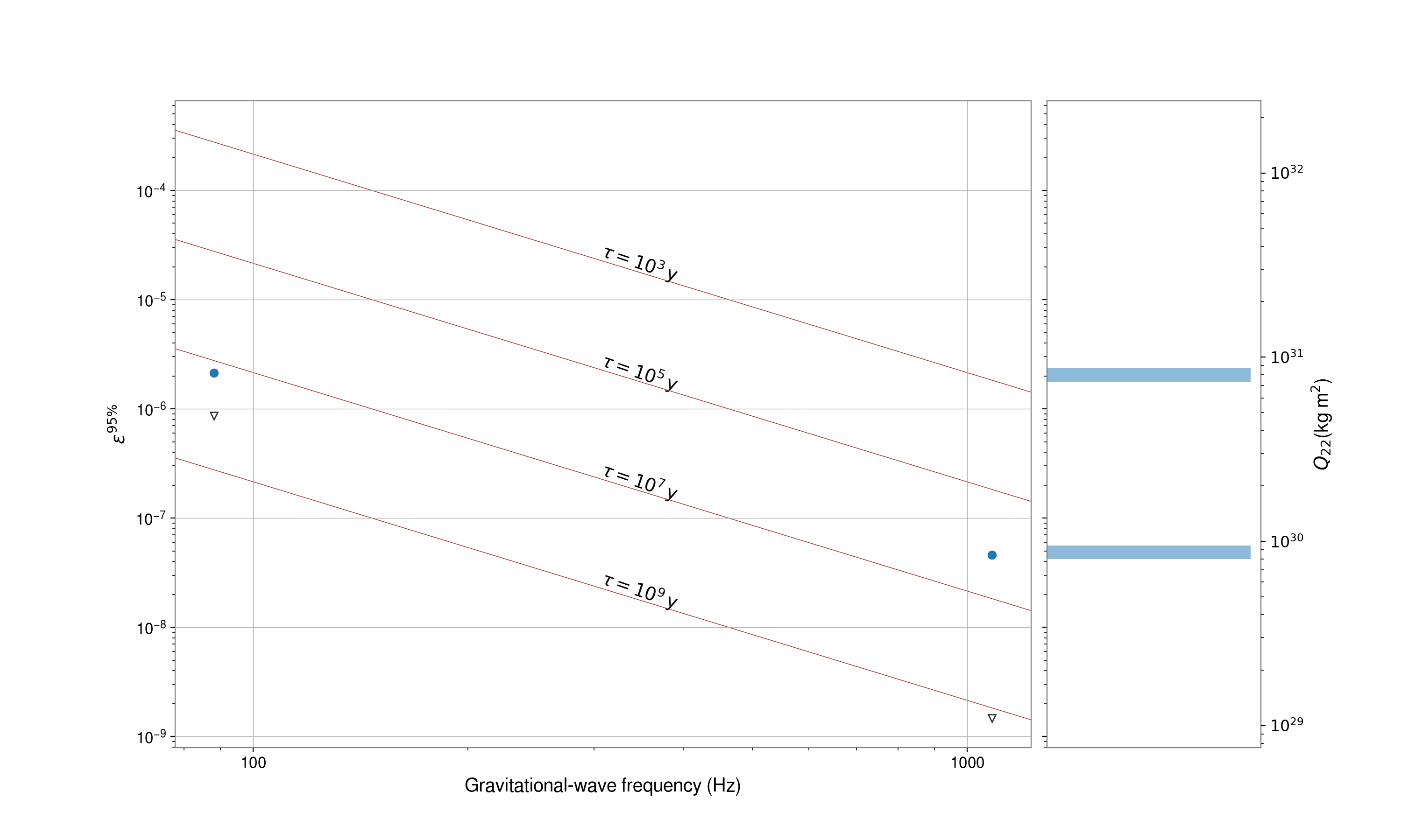
The plot() method of the UpperLimitTable can also be used to produce summary plots of the results, e.g., upper limits on \(h_0\) or ellipticity against signal frequency:

# get O2 amplitude spectral density estimates so we can overplot sensitivity estimates
import requests
import numpy as np
O2H1asd = "O2_H1_asd.txt"
O2H1obs = 158 * 86400  # 158 days
np.savetxt(
    O2H1asd,
    np.array([[float(val.strip()) for val in line.split()] for line in requests.get(
        "https://dcc.ligo.org/public/0156/G1801950/001/2017-06-10_DCH_C02_H1_O2_Sensitivity_strain_asd.txt"
    ).text.strip().split("\n")]),
)
O2L1asd = "O2_L1_asd.txt"
O2L1obs = 154 * 86400  # 154 days
np.savetxt(
    O2L1asd,
    np.array([[float(val.strip()) for val in line.split()] for line in requests.get(
        "https://dcc.ligo.org/public/0156/G1801952/001/2017-08-06_DCH_C02_L1_O2_Sensitivity_strain_asd.txt"
    ).text.strip().split("\n")]),
)

# plot h0 (by default this will use the joint H1L1V1 upper limits)
fig = tab.plot(
    column="h0",
    histogram=True,  # include a histogram of h0 values on rhs of plot
    showsdlim=True,  # show spin-down limits
    asds=[O2H1asd, O2L1asd],  # calculate and show sensitivity estimate
    tobs=[O2H1obs, O2L1obs],  # observing times for sensitivity estimate
)
fig.show()

# plot ellipticity upper limits
fig = tab.plot(
   column="ell",
   histogram=True,
   showsdlim=True,
   showq22=True,  # show axis including Q22 values
   showtau=True,  # add isocontour of constant characteristic age (for n=5)
)
fig.show()

Note

By default, if calculating limits on the ellipticity/spin-down ratio, the UpperLimitTable will attempt to get values for the pulsar’s distance and (intrinsic) frequency derivative using the values found in the ATNF Pulsar Catalogue. These values can be manually provided if necessary.

Searching for non-GR polarisation modes

The heterodyned output of the above pipeline can be re-used to perform a search for a signal that contains some combination of generic tensor, vector and scalar polarisation modes, i.e., a non-GR signal. This will assume that the signals are still emitted at twice the rotation frequency of the the pulsars. This will just use the cwinpy_pe_pipeline and a new prior file. An example configuration file for this can be downloaded here and is reproduced below:

[run]
basedir = /home/matthew.pitkin/projects/cwinpyO2

[pe_dag]
name = nongr_pe
submitdag = True

[pe_job]
accounting_group = ligo.prod.o2.cw.targeted.bayesian
accounting_group_user = matthew.pitkin

[ephemerides]
pulsars = /home/matthew.pitkin/projects/O2pulsars

[pe]
results = results_nongr
data-file-2f = {"H1": "/home/matthew.pitkin/projects/cwinpyO2/heterodyne/H1", "L1": "/home/matthew.pitkin/projects/cwinpyO2/heterodyne/L1"}
incoherent = True
priors = /home/matthew.pitkin/projects/O2priors/priors_nongr.txt

while a possible prior file might contain, e.g.,:

hplus = FermiDirac(1.0e-24, mu=1.0e-22, name='hplus')
hcross = FermiDirac(1.0e-24, mu=1.0e-22, name='h0')
phi0tensor = Uniform(minimum=0.0, maximum=2*pi, name='phi0tensor')
psitensor = Uniform(minimum=0.0, maximum=2*pi, name='psitensor')
hvectorx = FermiDirac(1.0e-24, mu=1.0e-22, name='hvectorx')
hvectory = FermiDirac(1.0e-24, mu=1.0e-22, name='hvectory')
phi0vector = Uniform(minimum=0.0, maximum=2*pi, name='phi0vector')
psivector = Uniform(minimum=0.0, maximum=2*pi, name='psivector')
hscalarb = FermiDirac(1.0e-24, mu=1.0e-22, name='hscalarb')
phi0scalar = Uniform(minimum=0.0, maximum=2*pi, name='phi0scalar')
psiscalar = Uniform(minimum=0.0, maximum=2*pi, name='psiscalar')

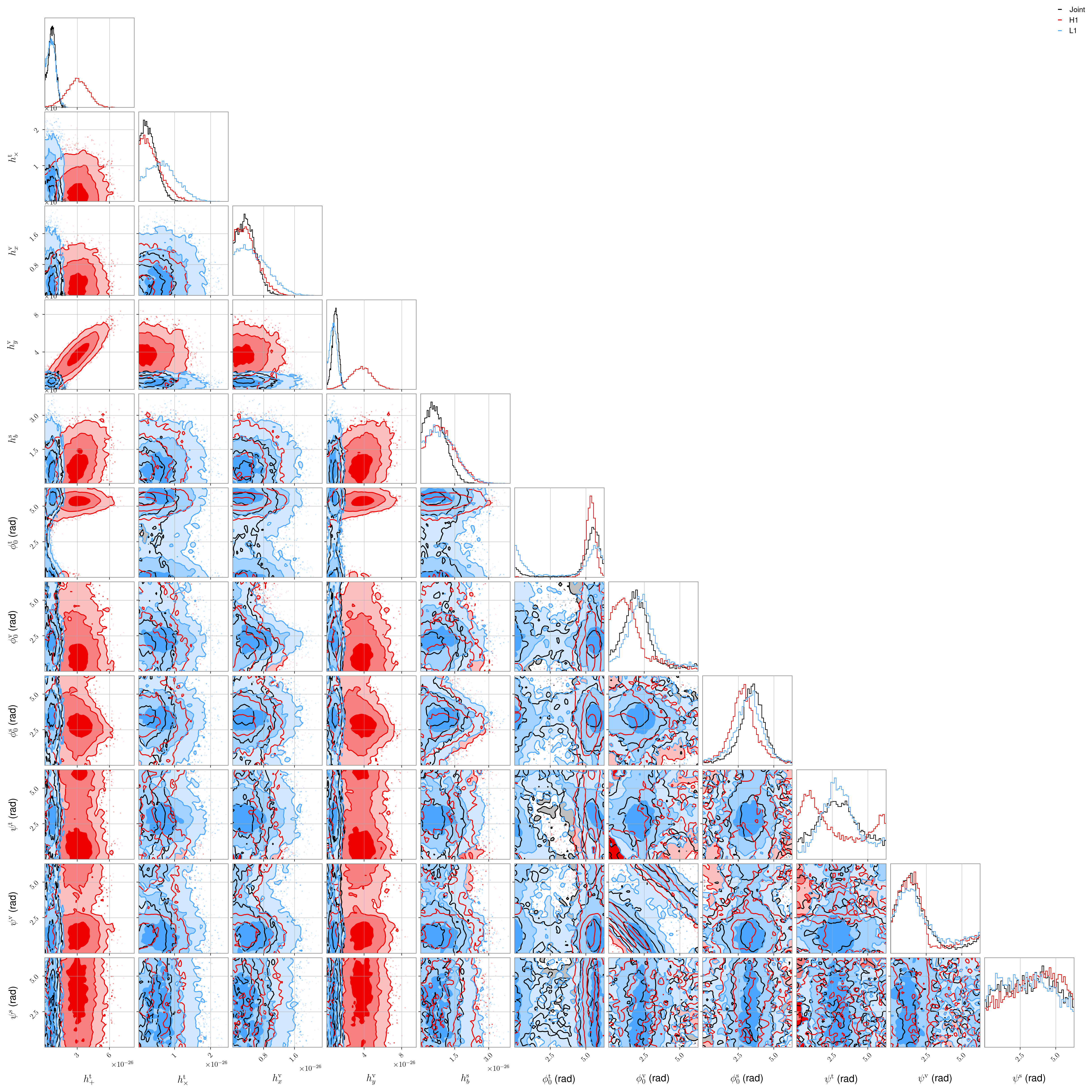
In this case, the prior assumes a signal containing tensor (hplus and hcross), vector (hvectorx and hvectory) and scalar (hscalarb, but not hscalarl as they are completely degenerate) amplitudes and associated initial phases and polarisations. The phases and polarisation all cover a \(2\pi\) radian range.

This would be run with:

$ cwinpy_pe_pipeline cwinpy_pe_example_O2_nongr.ini

The analysis will take significantly longer (10s of hours) than the default analysis, which assumes just four unknown parameters.

This could have been achieved using the original cwinpy_knope_pipeline by passing it the non-GR prior file.

We can look at a plot for one of the pulsars showing the posteriors for all parameters for each detector with:

from cwinpy.plot import Plot

plot = Plot(
    {
        "Joint": "J0737-3039A/cwinpy_pe_H1L1_J0737-3039A_result.hdf5",
        "H1": "J0737-3039A/cwinpy_pe_H1_J0737-3039A_result.hdf5",
        "L1": "J0737-3039A/cwinpy_pe_L1_J0737-3039A_result.hdf5",
    },
    parameters=[
        "hplus",
        "hcross",
        "hvectorx",
        "hvectory",
        "hscalarb",
        "phi0tensor",
        "phi0vector",
        "phi0scalar",
        "psitensor",
        "psivector",
        "psiscalar"
    ]
)

plot.plot()
plot.fig.show()

O3 LIGO/Virgo (proprietary) data, dual harmonic

An example configuration file for performing a search for multiple pulsars, for a signal with components a both the rotation frequency and twice the rotation frequency (the \(l=2,m=1\) and the \(l=m=2\) harmonics), using proprietary O3 LIGO and Virgo data can be downloaded here and is reproduced below:

[run]
basedir = /home/matthew.pitkin/projects/cwinpyO3

[knope_job]
accounting_group = ligo.prod.o3.cw.targeted.bayesian
accounting_group_user = matthew.pitkin

[ephemerides]
pulsarfiles = /home/matthew.pitkin/projects/O3pulsars
earth = {"DE436": "/home/matthew.pitkin/projects/ephemerides/earth00-40-DE436.dat.gz"}
sun = {"DE436": "/home/matthew.pitkin/projects/ephemerides/sun00-40-DE436.dat.gz"}

[heterodyne]
detectors = ["H1", "L1", "V1"]
freqfactors = [1, 2]
starttimes = 1238166018
endtimes = 1269363618
frametypes = {"H1": "H1_HOFT_C01", "L1": "L1_HOFT_C01", "V1": "V1Online"}
channels = {"H1": "H1:DCS-CALIB_STRAIN_C01", "L1": "L1:DCS-CALIB_STRAIN_C01", "V1": "V1:Hrec_hoft_16384Hz"}
host = datafind.ligo.org:443
includeflags = {"H1": "H1:DCS-ANALYSIS_READY_C01:1", "L1": "L1:DCS-ANALYSIS_READY_C01:1", "V1": "V1:ITF_SCIENCE:2"}
excludeflags = {"H1": "H1:DCS-MISSING_H1_HOFT_C01:1", "L1": "L1:DCS-MISSING_L1_HOFT_C01:1", "V1": "V1:DQ_HREC_MISSING_V1ONLINE,V1:DQ_HREC_IS_ZERO,V1:DQ_HREC_BAD_QUALITY"}
outputdir = {"H1": "/home/matthew.pitkin/projects/cwinpyO3/heterodyne/H1", "L1": "/home/matthew.pitkin/projects/cwinpyO3/heterodyne/L1", "V1": "/home/matthew.pitkin/projects/cwinpyO3/heterodyne/V1"}

[merge]
remove = True

[pe_dag]
submitdag = True

[pe]
n_parallel = 2
sampler-kwargs = {"nlive": 500}
incoherent = True

This requires the parameters for the pulsar to be within the /home/matthew.pitkin/projects/O3pulsars directory (in the example results shown below this directory contained files for the two pulsars J0437-4715 and J0771-6830). In this example the default priors and used, so no prior file is explicitly given.

The pulsar parameter files used in the example were generated using the DE436 solar system ephemeris, which is not one of the default files available within LALSuite. Therefore, these have had to be generated using the commands:

$ lalpulsar_create_solar_system_ephemeris_python --target SUN --year-start 2000 --interval 20 --num-years 40 --ephemeris DE436 --output-file sun00-40-DE436.dat
$ lalpulsar_create_solar_system_ephemeris_python --target EARTH --year-start 2000 --interval 2 --num-years 40 --ephemeris DE436 --output-file earth00-40-DE436.dat

and then gzipped. Alternatively, the usetempo2 option could be used, where the latest TEMPO2 version will contain these ephemerides.

This would be run with:

$ cwinpy_knope_pipeline knope_example_O3_dual.ini

Note

If running on open GWOSC data, the O3a and O3b periods need to be treated as separate runs as in the above example. This is automatically dealt with if setting up a cwinpy_knope_pipeline run using the “Quick setup”.

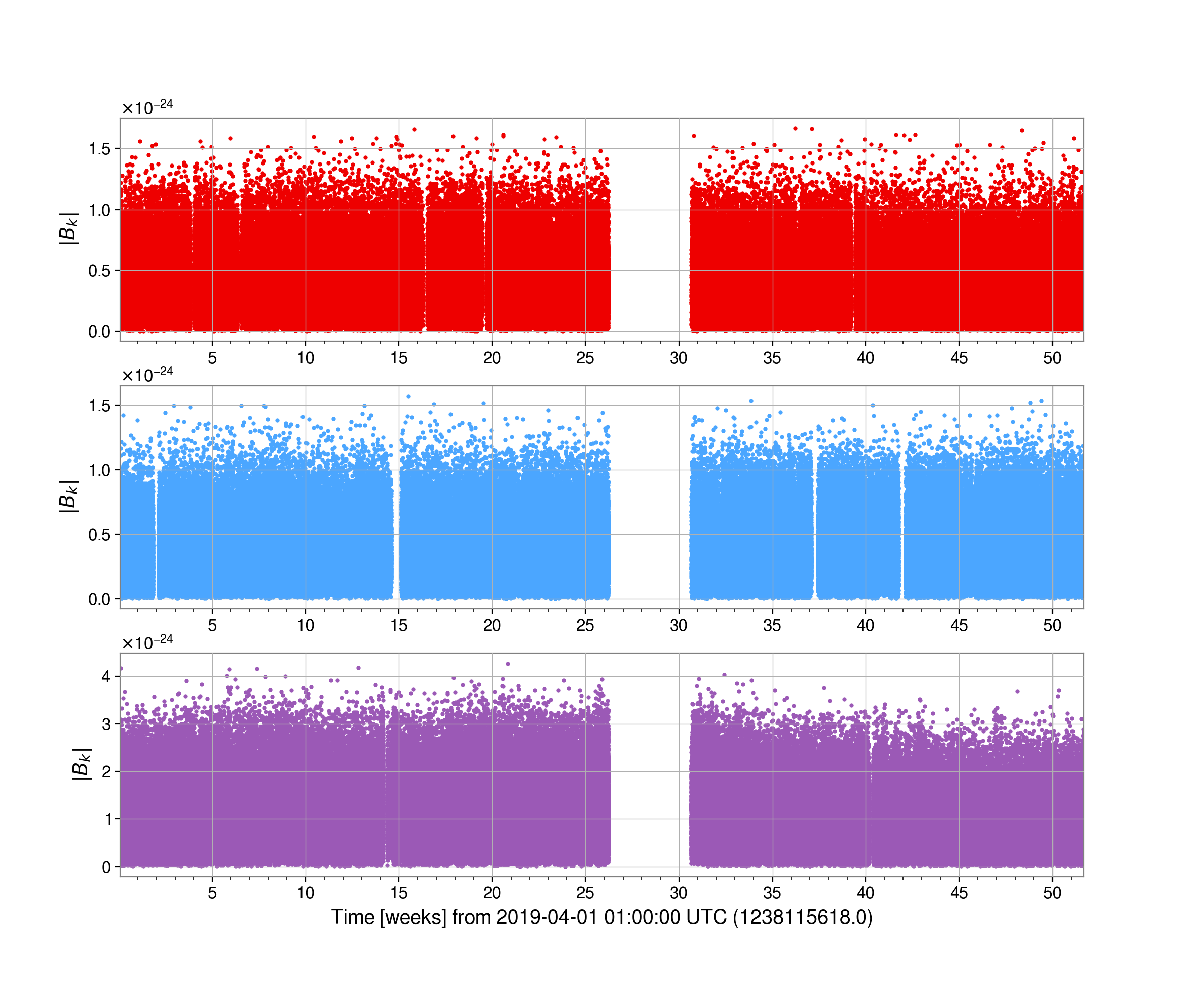
Once complete, this example should have generated the heterodyned data files for H1, L1 and V1 (within the /home/matthew.pitkin/projects/cwinpyO3/heterodyne directory) for the signals at both once and twice the pulsar rotation frequency.

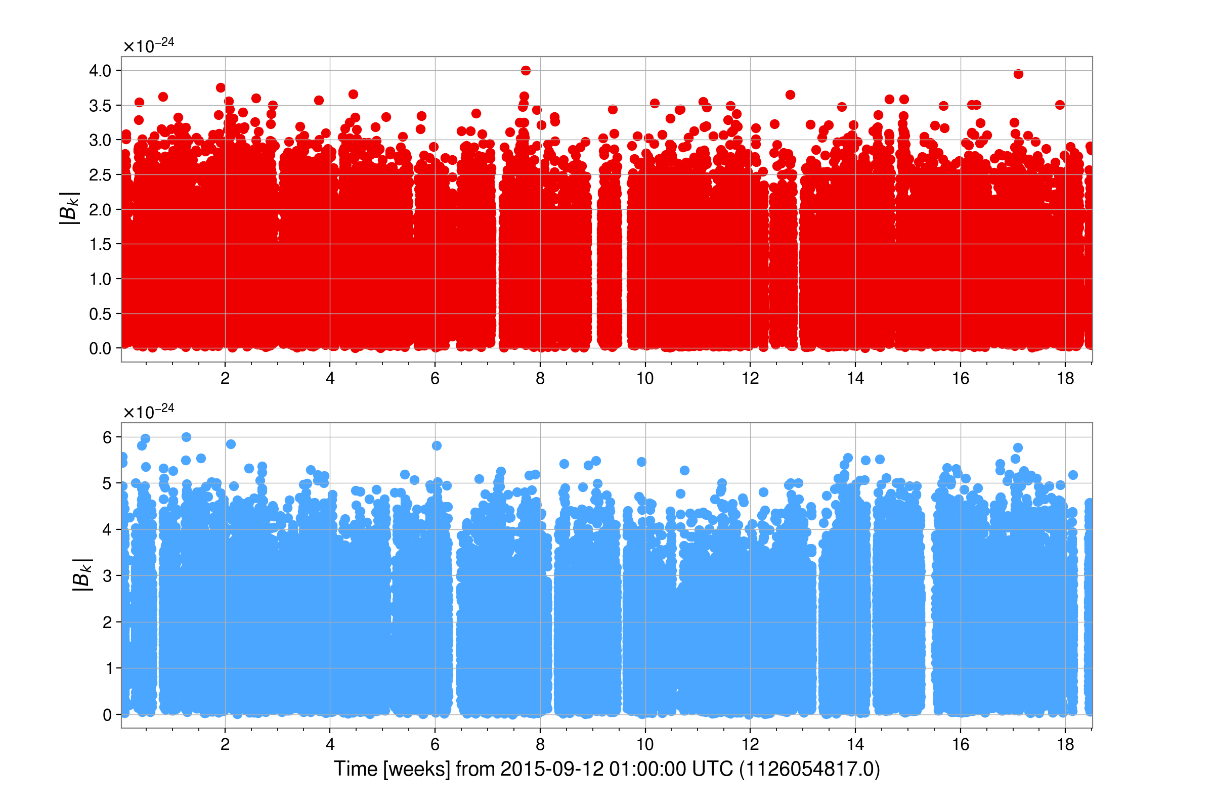
We could look at the heterodyned data at the rotation frequency for the pulsar J0437-4715 using:

from cwinpy import MultiHeterodynedData

het = MultiHeterodynedData(
   {
       "H1": "H1/heterodyne_J0437-4715_H1_1_1238166018-1269363618.hdf5",
       "L1": "L1/heterodyne_J0437-4715_L1_1_1238166018-1269363615.hdf5",
       "V1": "V1/heterodyne_J0437-4715_V1_1_1238166018-1269363618.hdf5",
   }
)

fig = het.plot(together=True, remove_outliers=True, markersize=2)
fig.show()

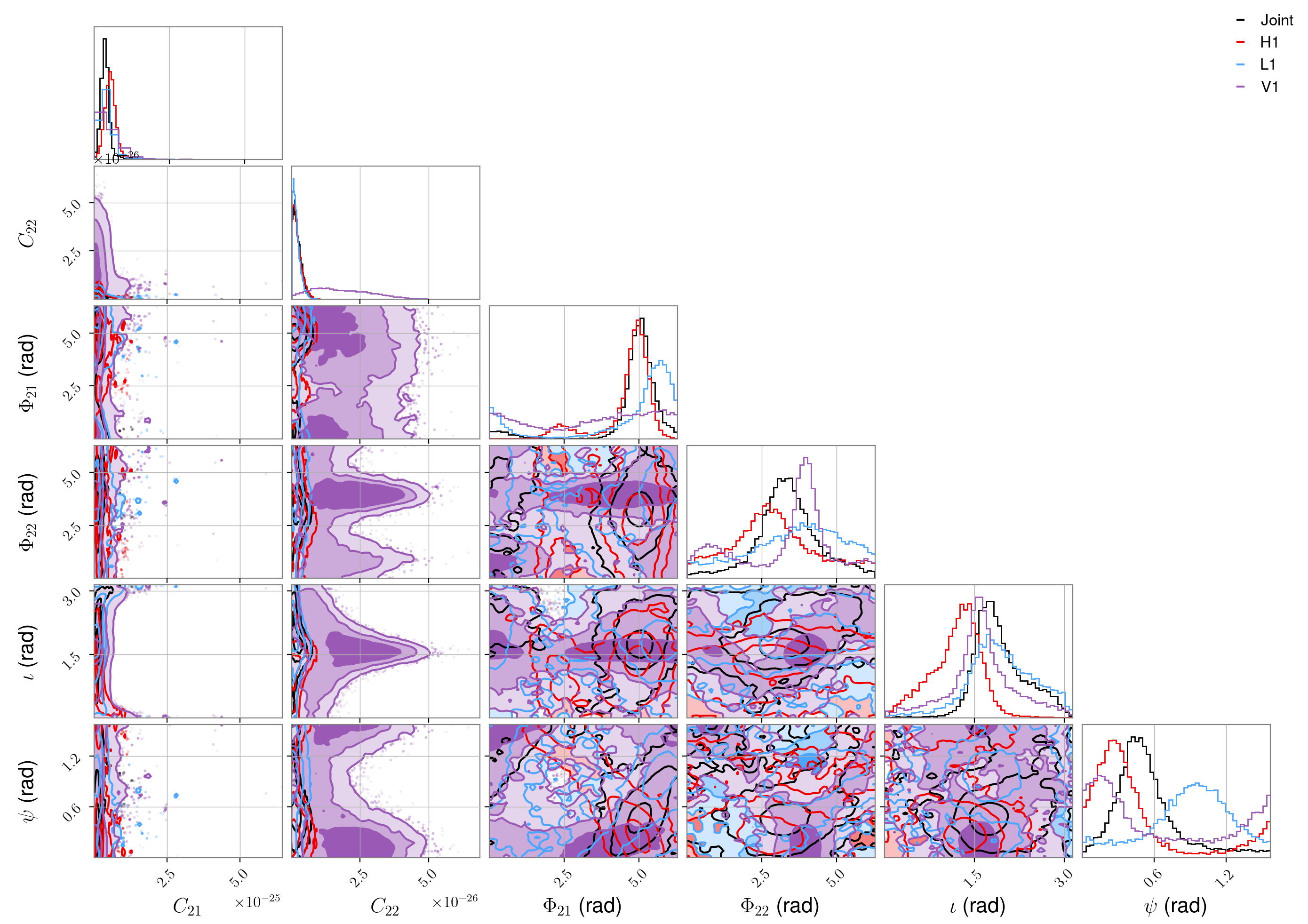
The results of the parameter estimation stage would be found in the /home/matthew.pitkin/projects/cwinpyO3/results directory. Posteriors parameter distributions for all the parameters for J0437-4715, for each detector and the joint detector analysis, could be plotted using:

from cwinpy.plot import Plot

plot = Plot(
    {
        "Joint": "J0437-4715/cwinpy_pe_H1L1V1_J0437-4715_result.hdf5",
        "H1": "J0437-4715/cwinpy_pe_H1_J0437-4715_result.hdf5",
        "L1": "J0437-4715/cwinpy_pe_L1_J0437-4715_result.hdf5",
        "V1": "J0437-4715/cwinpy_pe_V1_J0437-4715_result.hdf5",
    },
    parameters=[
        "c21",
        "c22",
        "phi21",
        "phi22",
        "iota",
        "psi",
    ]
)

plot.plot()
plot.fig.show()

O2 LIGO (open) data, “transient-continuous” signal following a pulsar glitch

As described in this example, the signal model used by CWInPy can be one that is described as “transient-continuous” (see., e.g., [1] and [2]). Unlike the standard signal that is assumed to be “always on”, the transient-continuous signal is modulated by a window function; currently this can consist of a rectangular window, i.e., the signal abruptly turns of and then off, or an exponential window, i.e., the signal turns on and then the amplitude decays away exponentially. Such a signal might occur after an event such as a pulsar glitch, which could “raise a mountain” on the star that subsequently decays away on a timescale of days-to-weeks-to-months [3].

An example configuration file for performing a search for such a signal is given below. In this case it uses open LIGO data from the O2 observing run to search for an exponentially decaying signal following a glitch observed in the Vela pulsar on 12 December 2016 [4].

[run]
basedir = /home/matthew.pitkin/projects/vela

[knope_job]
accounting_group = ligo.prod.o2.cw.targeted.bayesian
accounting_group_user = matthew.pitkin

[ephemerides]
pulsarfiles = /home/matthew.pitkin/projects/vela/vela.par

[heterodyne]
detectors = ["H1", "L1"]
freqfactors = 2
starttimes = 1164556817
endtimes = 1187733618
frametypes = {"H1": "H1_GWOSC_O2_4KHZ_R1", "L1": "L1_GWOSC_O2_4KHZ_R1"}
channels = {"H1":"H1:GWOSC-4KHZ_R1_STRAIN", "L1": "L1:GWOSC-4KHZ_R1_STRAIN"}
host = datafind.gwosc.org
includeflags = {"H1": "H1_CBC_CAT1", "L1": "L1_CBC_CAT1"}
outputdir = {"H1": "/home/matthew.pitkin/projects/vela/heterodyne/H1", "L1": "/home/matthew.pitkin/projects/vela/heterodyne/L1"}
usetempo2 = False

[merge]
remove = True

[pe_dag]
submitdag = True

[pe]
priors = /home/matthew.pitkin/projects/vela/vela_transient_prior.txt
incoherent = True

Unlike in the O2 example above, this does not use data from the Virgo detector as that only covers the end of the O2 run, which will be well past the assumed transient timescale. This example assumes that you have a file (vela.par) containing the ephemeris for the Vela pulsar from radio observations overlapping the O2 run. To use the transient-continuous model, this file needs to contain a line defining the transient window type, in this case an exponential:

TRANSIENTWINDOWTYPE EXP

The example also needs a prior file (vela_transient_prior.txt) which contains the priors on the parameters of the window: the start time (taken to be close to the observed glitch time) and the decay time constant. If following the analysis of [2], the prior on the signal start time can be ±0.5 days either side of the observed glitch time (this is actually much larger than the uncertainty on the glitch time), which is at an MJD of 57734.4849906 (or GPS(TT) time of 1165577852). The signal decay time here is set from to be from 1.5 days to 150. An example of such a prior to use is:

h0 = FermiDirac(1.0e-24, mu=1.0e-22, name='h0', latex_label='$h_0$')
phi0 = Uniform(minimum=0.0, maximum=pi, name='phi0', latex_label='$\phi_0$', unit='rad')
iota = Sine(minimum=0.0, maximum=pi, name='iota', latex_label='$\iota$', unit='rad')
psi = Uniform(name='psi', minimum=0, maximum=np.pi / 2, latex_label='$\psi$', unit='rad')
transientstarttime = Uniform(name='transientstarttime', minimum=57733.9849906, maximum=57734.9849906, latex_label='$t_0$', unit='d')
transienttau = Uniform(name='transienttau', minimum=1.5, maximum=150, latex_label='$\\tau$', unit='d')

Note

If setting the transientstarttime and transienttau prior values using MJD and days, respectively, the unit keyword of the prior must be set to 'd', otherwise the start time will be assumed to be a GPS time and the decay timescale will be assumed to be in seconds.

This would be run with:

$ cwinpy_knope_pipeline knope_example_O2_vela_transient.ini

The results of the parameter estimation stage would be found in the /home/matthew.pitkin/projects/vela/results directory. Posteriors parameter distributions for all the parameters, including the transient parameters, for each detector and the joint detector analysis, could be plotted using:

from cwinpy.plot import Plot

plot = Plot(
    {
        "Joint": "J0835-4510/cwinpy_pe_H1L1_J0835-4510_result.hdf5",
        "H1": "J0835-4510/cwinpy_pe_H1_J0835-4510_result.hdf5",
        "L1": "J0835-4510/cwinpy_pe_L1_J0835-4510_result.hdf5",
    },
    parameters=[
        "h0",
        "phi0",
        "iota",
        "psi",
        "transientstarttime",
        "transienttau",
    ]
)

plot.plot()
plot.fig.show()

# output 95% upper limits on h0
plot.upper_limit("h0", 0.95)

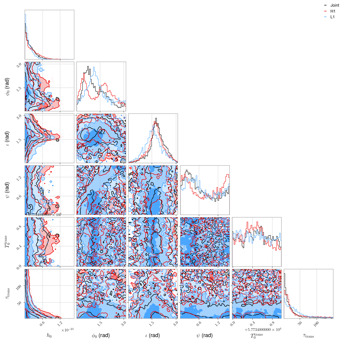
The 95% credible upper limits on \(h_0\) in this case are:

• H1: \(6.8\!\times\!10^{-24}\)

• L1: \(4.1\!\times\!10^{-24}\)

• Joint (H1 & L1): \(5.3\!\times\!10^{-24}\)

It is interesting to see that there is a strong correlation between \(h_0\) and the transient decay time constant \(\tau_{\rm{trans}}\), with a broader distribution of \(h_0\) associated with smaller values of \(\tau_{\rm{trans}}\). This is expected, as you would expect to be more sensitive to longer signals.

Generating results webpages

If you have run the cwinpy_knope_pipeline, it will generate a version of the input configuration file within the analysis directory called knope_pipeline_config.ini. After the analysis is complete, i.e., the HTCondor DAG has successfully run, this configuration file can be used as an input for generating a set of results pages. These pages (based on PESummary [5]) will display summary tables and plots of the results for all sources, e.g., upper limits on the gravitational-wave amplitude, as well as pages with information and posterior plots for each individual pulsar.

These pages can be generated using the cwinpy_generate_summary_pages command line interface script or the generate_summary_pages() API, which give control over what information is generated and output.

For example, to generate summary webpages that include a table of upper limits on gravitational-wave amplitude, plots of these limits (also after converting to equivalent limits on the each pulsar’s ellipticity and mass quadrupole moment), estimates of the signal-to-noise ratio and Bayesian odds, and individual pages for each pulsar, one could just run:

$ cwinpy_generate_summary_pages --outpath /home/albert.einstein/public_html/analysis \
--url https://ldas-jobs.ligo.caltech.edu/~albert.einstein/analysis \
knope_pipeline_config.ini

where --outpath points to the path of a web-accessible directory and --url gives the associated URL of that directory (for URLs for the user webpage for each LDG cluster, see the appropriate cluster listed here and look for the “User webspace”; currently the URL is not actually used, so a dummy string can be passed). If you have many sources, this could takes tens of minutes to run.

Warning

The webpage generation scripts are currently not included in the CWInPy test suite and as such the interface may be buggy.

knope Command line arguments

The command line arguments for cwinpy_knope can be found using:

$ cwinpy_knope --help
usage: cwinpy_knope [-h] --heterodyne-config HETERODYNE_CONFIG --pe-config
                    PE_CONFIG [--version]

A script to run the CWInPy known pulsar analysis pipeline; gravitational-wave
data will be preprocessed based on the phase evolution of a pulsar which will
then be used to infer the unknown signal parameters.

optional arguments:
  -h, --help            show this help message and exit
  --heterodyne-config HETERODYNE_CONFIG
                        A configuration file for the heterodyne pre-processing
                        using cwinpy_heterodyne. If requiring multiple
                        detectors then this option can be used multiple times
                        to pass configuration files for each detector.
  --pe-config PE_CONFIG
                        A configuration file for the Bayesian inference stage
                        using cwinpy_pe.
  --version             show program's version number and exit

The command line arguments for cwinpy_knope_pipeline can be found using:

$ cwinpy_knope_pipeline --help
usage: cwinpy_knope_pipeline [-h] [--run RUN] [--detector DETECTOR] [--hwinj]
                             [--samplerate SAMPLERATE] [--pulsar PULSAR]
                             [--osg] [--output OUTPUT] [--joblength JOBLENGTH]
                             [--include-incoherent] [--incoherent-only]
                             [--accounting-group ACCGROUP] [--usetempo2]
                             [config]

A script to create a HTCondor DAG to process GW strain data by heterodyning it
based on the expected phase evolution for a selection of pulsars, and then
perform parameter estimation for the unknown signal parameters of those
sources.

positional arguments:
  config                The configuration file for the analysis

optional arguments:
  -h, --help            show this help message and exit

Quick setup arguments (this assumes CVMFS open data access).:
  --run RUN             Set an observing run name for which to heterodyne the
                        data. This can be one of S5, S6, O1, O2, O3a, O3b, O3
                        for which open data exists
  --detector DETECTOR   The detector for which the data will be heterodyned.
                        This can be used multiple times to specify multiple
                        detectors. If not set then all detectors available for
                        a given run will be used.
  --hwinj               Set this flag to analyse the continuous hardware
                        injections for a given run. No '--pulsar' arguments
                        are required in this case, in which case all hardware
                        injections will be used. To specific particular
                        hardware injections, the required names can be set
                        with the '--pulsar' flag.
  --samplerate SAMPLERATE
                        Select the sample rate of the data to use. This can
                        either be 4k or 16k for data sampled at 4096 or 16384
                        Hz, respectively. The default is 4k, except if running
                        on hardware injections for O1 or later, for which 16k
                        will be used due to being required for the highest
                        frequency source. For the S5 and S6 runs only 4k data
                        is available from GWOSC, so if 16k is chosen it will
                        be ignored.
  --pulsar PULSAR       The path to a TEMPO(2)-style pulsar parameter file, or
                        directory containing multiple parameter files, to
                        heterodyne. This can be used multiple times to specify
                        multiple pulsar inputs. If a pulsar name is given
                        instead of a parameter file then an attempt will be
                        made to find the pulsar's ephemeris from the ATNF
                        pulsar catalogue, which will then be used.
  --osg                 Set this flag to run on the Open Science Grid rather
                        than a local computer cluster.
  --output OUTPUT       The location for outputting the heterodyned data. By
                        default the current directory will be used. Within
                        this directory, subdirectories for each detector will
                        be created.
  --joblength JOBLENGTH
                        The length of data (in seconds) into which to split
                        the individual analysis jobs. By default this is set
                        to 86400, i.e., one day. If this is set to 0, then the
                        whole dataset is treated as a single job.
  --include-incoherent  If running with multiple detectors, set this flag to
                        analyse each of them independently and also include an
                        analysis that coherently combines the data from all
                        detectors. Only performing a coherent analysis is the
                        default.
  --incoherent-only     If running with multiple detectors, set this flag to
                        analyse each of them independently rather than
                        coherently combining the data from all detectors. Only
                        performing a coherent analysis is the default.
  --accounting-group ACCGROUP
                        For LVK users this sets the computing accounting group
                        tag
  --usetempo2           Set this flag to use Tempo2 (if installed) for
                        calculating the signal phase evolution for the
                        heterodyne rather than the default LALSuite functions.

Knope API

knope(**kwargs)

Run the known pulsar pipeline within Python. It is highly recommended to run the pipeline script cwinpy_knope_pipeline to create a HTCondor DAG, particular if using data from a long observing run and/or for multiple pulsars. The main use of this function is for quick testing.

This interface can be used for analysing data from multiple detectors or multiple harmonics by passing multiple heterodyne configuration settings for each case, but this is not recommended.

Parameters:

• heterodyne_config (str, list) – The path to a configuration file, or list of paths to multiple configuration files if using more than one detector, of the type required by cwinpy_heterodyne.

• hetkwargs (dict, list) – If not using a configuration file, arguments for cwinpy.heterodyne.heterodyne() can be provided as a dictionary, or list of dictionaries if requiring more than one detector.

• pe_config (str) – The path to a configuration file of the type required by cwinpy_pe. The input data arguments and pulsars used will be assumed to be the same as for the heterodyne configuration file, so any values given in the configuration file will be ignored.

• pekwargs (dict) – If not using a configuration file, arguments for cwinpy.pe.pe() can be provided as a dictionary.

Returns:

The returned values are a dictionary containing lists of the cwinpy.heterodyne.Heterodyne objects produced during heterodyning (keyed by frequency scale factor) and a dictionary (keyed by pulsar name) containing bilby.core.result.Result objects for each pulsar.

Return type:

tuple

knope_pipeline(**kwargs)

Run knope within Python. This will create a HTCondor DAG for consecutively running multiple cwinpy_heterodyne and cwinpy_pe instances on a computer cluster. Optional parameters that can be used instead of a configuration file (for “quick setup”) are given in the “Other parameters” section.

Parameters:

config (str) – A configuration file, or configparser:ConfigParser object, for the analysis.

Other Parameters:

• run (str) – The name of an observing run for which open data exists, which will be heterodyned, e.g., “O1”.

• detector (str, list) – The detector, or list of detectors, for which the data will be heterodyned. If not set then all detectors available for a given run will be used.

• hwinj (bool) – Set this to True to analyse the continuous hardware injections for a given run. If no pulsar argument is given then all hardware injections will be analysed. To specify particular hardware injections the names can be given using the pulsar argument.

• samplerate (str:) – Select the sample rate of the data to use. This can either be 4k or 16k for data sampled at 4096 or 16384 Hz, respectively. The default is 4k, except if running on hardware injections for O1 or later, for which 16k will be used due to being required for the highest frequency source. For the S5 and S6 runs only 4k data is available from GWOSC, so if 16k is chosen it will be ignored.

• pulsar (str, list) – The path to, or list of paths to, a TEMPO(2)-style pulsar parameter file(s), or directory containing multiple parameter files, to heterodyne. If a pulsar name is given instead of a parameter file then an attempt will be made to find the pulsar’s ephemeris from the ATNF pulsar catalogue, which will then be used.

• osg (bool) – Set this to True to run on the Open Science Grid rather than a local computer cluster.

• output (str) – The base location for outputting the heterodyned data and parameter estimation results. By default the current directory will be used. Within this directory, subdirectories for each detector and for the result swill be created.

• joblength (int) – The length of data (in seconds) into which to split the individual heterodyne jobs. By default this is set to 86400, i.e., one day. If this is set to 0, then the whole dataset is treated as a single job.

• accounting_group (str) – For LVK users this sets the computing accounting group tag.

• usetempo2 (bool) – Set this flag to use Tempo2 (if installed) for calculating the signal phase evolution for the heterodyne rather than the default LALSuite functions.

• includeincoherent (bool) – If using multiple detectors, as well as running an analysis that coherently combines data from all given detectors, also analyse each individual detector’s data separately. The default is False, i.e., only the coherent analysis is performed.

• incoherentonly (bool) – If using multiple detectors, only perform analyses on the individual detector’s data and do not analyse a coherent combination of the detectors.

Returns:

An object containing a pycondor pycondor.Dagman object.

Return type:

dag

generate_summary_pages(**kwargs)

Generate summary webpages following a cwinpy_knope_pipeline analysis (see knope_pipeline()).

Parameters:

• config (str, Path) – The configuration file used for the cwinpy_knope_pipeline analysis.

• outpath (str, Path) – The output path for the summary results webpages and plots.

• url (str) – The URL from which the summary results pages will be accessed.

• showposteriors (bool) – Set to enable/disable production of plots showing the joint posteriors for all parameters. The default is True.

• showindividualposteriors (bool) – Set to enable/disable production of plots showing the marginal posteriors for each individual parameter. The default is False.

• showtimeseries (bool) – Set to enable/disable production of plots showing the heterodyned time series data (and spectral representations). The default is True.

• pulsars (list, str) – A list of pulsars to show. By default all pulsars analysed will be shown.

• upperlimitplot (bool) – Set to enable/disable production of plots of amplitude upper limits as a function of frequency. The default is True.

• oddsplot (bool) – Set to enable/disable production of plots of odds vs SNR and frequency. The default is True.

• showsnr (bool) – Set to calculate and show the optimal matched filter signal-to-noise ratio for the recovered maximum a-posteriori waveform. The default is False.

• showodds (bool) – Set to calculate and show the log Bayesian odds for the coherent signal model vs. noise/incoherent signals. The default is False.

• sortby (str) – Set the parameter on which to sort the table of results. The allowed parameters are: ‘PSRJ’, ‘F0’, ‘F1’, ‘DIST’, ‘H0’, ‘H0SPINDOWN’, ‘ELL’, ‘Q22’, ‘SDRAT’, and ‘ODDS’. When sorting on upper limits, if there are multiple detectors, the results from the detector with the most constraining limit will be sorted on.

• sortdescending (bool) – By default the table of results will be sorted in ascending order on the chosen parameter. Set this argument to True to instead sort in descending order.

• onlyjoint (bool) – By default all single detector and multi-detector (joint) analysis results will be tabulated if present. Set this argument to True to instead only show the joint analysis in the table of results.

• onlymsps (bool) – Set this flag to True to only include recycled millisecond pulsars in the output. We defined an MSP as having a rotation period less than 30 ms (rotation frequency greater than 33.3 Hz) and an estimated B-field of less than 1e11 Gauss.

Knope references

[1]

R. Prix, S. Giampanis, S. & C. Messenger, C., PRD, 84, 023007 (2011)

[2] (1,2)

D. Keitel et al., PRD, 100, 064058 (2019)

[3]

G. Yim & D. I. Jones, MNRAS, 498, 3138-3152 (2020)

[4]

J. Palfreyman, Astron. Telegram, 9847 (2016)

[5]

C. Hoy & V. Raymond, SoftwareX, 15, 100765 (2021)