Code comparison#
Here we document comparisons between the analysis produced using CWInPy compared with the LALSuite code lalpulsar_parameter_estimation_nested (formerly
lalapps_pulsar_parameter_estimation_nested), and the full pipeline generation code
lalpulsar_knope (formerly lalapps_knope), which are described in [1].
The codes will be run on identical data and in configurations that are as close as possible.
Parameter estimation comparison#
Links to the various direct comparisons of pulsar parameter estimation are given below:
- Single detector, noise-only
- Single detector, software injection (linear polarisation)
- Single detector, software injection (circular polarisation)
- Multiple detectors, noise-only
- Multiple detectors, software injection (linear polarisation)
- Multiple detectors, software injection (circular polarisation)
- Single detector, noise-only, two harmonics
- Single detector, software injection, two harmonics
- Single detector, O1 data
- Single detector, O1 data (restricted prior)
- Single detector, O1 data, hardware injection
- Multiple detectors, O1 data
- Multiple detectors, O1 data, hardware injection
Posterior credible interval checks#
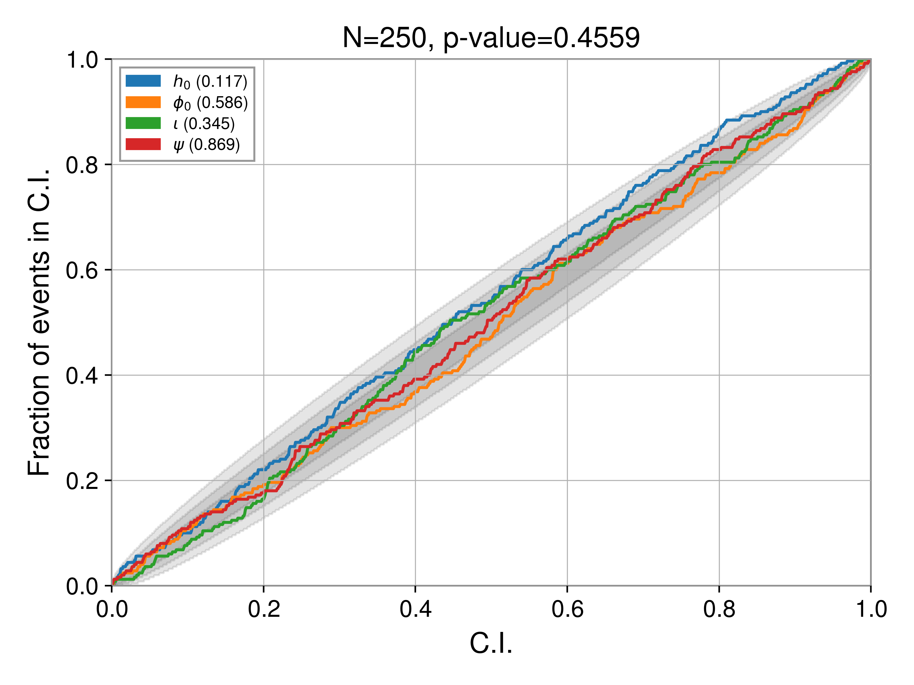
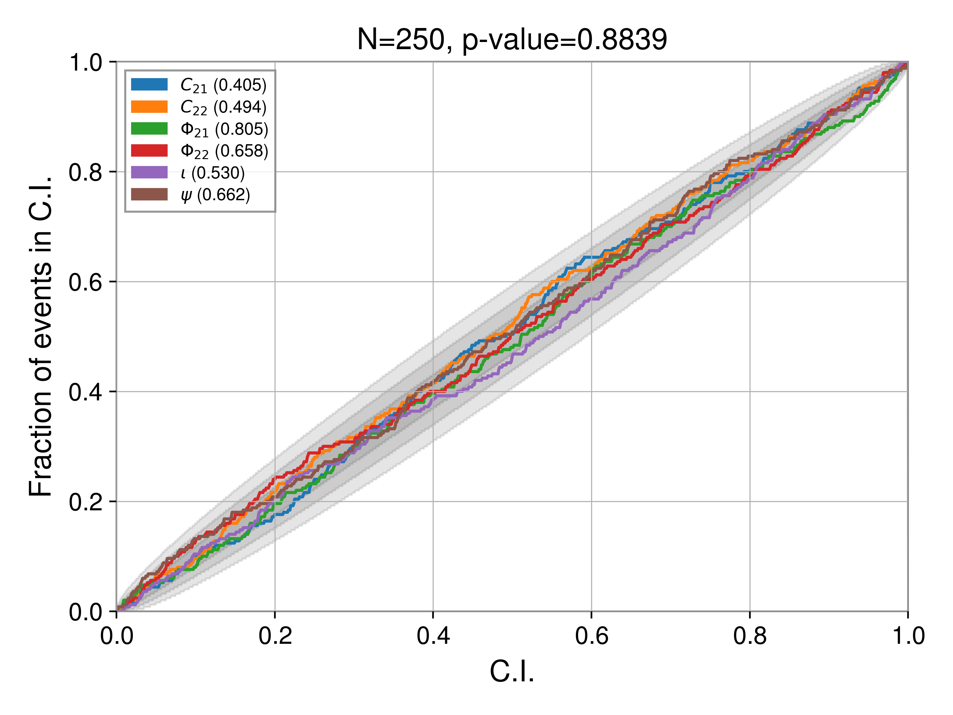
Another test of the code is to check that the posterior credible intervals resulting from any analysis correctly ascribe probability, i.e., that they are “well calibrated” [2]. To do this one can create a set of simulated signals with true parameters drawn from a particular prior, and then use the code to sample the posterior probability distribution over the parameter space for each parameter using the same prior. Using the one-dimensional marginalised posteriors for each parameter, and each simulation, one can then find the credible interval in which the known true signal parameter lies. If the credible intervals are correct you would expect, e.g., to find the true parameter in the 1% credible interval for 1% of the simulations, the true parameter within the 50% credible interval for 50% of the simulations, etc. A plot of the credible interval versus the percentage of true signal values found within that credible interval is known within the gravitational-wave community colloquially as a “PP plot” (see, e.g., Section VC of [3]). This is also more generally known as “Simulated-based calibration” [4].
These tests have been performed on the output of cwinpy_pe by generating a set of simulated
signals (using the cwinpy.pe.testing.PEPPPlotsDAG) to be analysed. After all the
individual simulations have been analysed, a PP plot is generated using
cwinpy.pe.testing.generate_pp_plots() (which itself uses functions from bilby).
Single harmonic signal#
We produce PP plots for the case of a signal from the \(l=m=2\) mass quadrupole of a pulsar,
where emission would be at twice the rotation frequency and defined by the parameters \(h_0\),
\(\phi_0\), \(\iota\) and \(\psi\). A Python file to run such an analysis for 250
simulated signals using PEPPPlotsDAG is shown below. This also
shows the priors used for the generation of signal parameters and their recovery.
Note
When drawing parameters from the \(h_0\) prior, a maximum cut-off (maxamp in the code)
that is lower than the upper range of the prior is used. This is to ensure that posteriors are
not truncated by the upper end of the prior in this case. However, this should not bias the
recovered credible intervals due to the \(h_0\) prior being uniform and extending well above
the maxamp value.
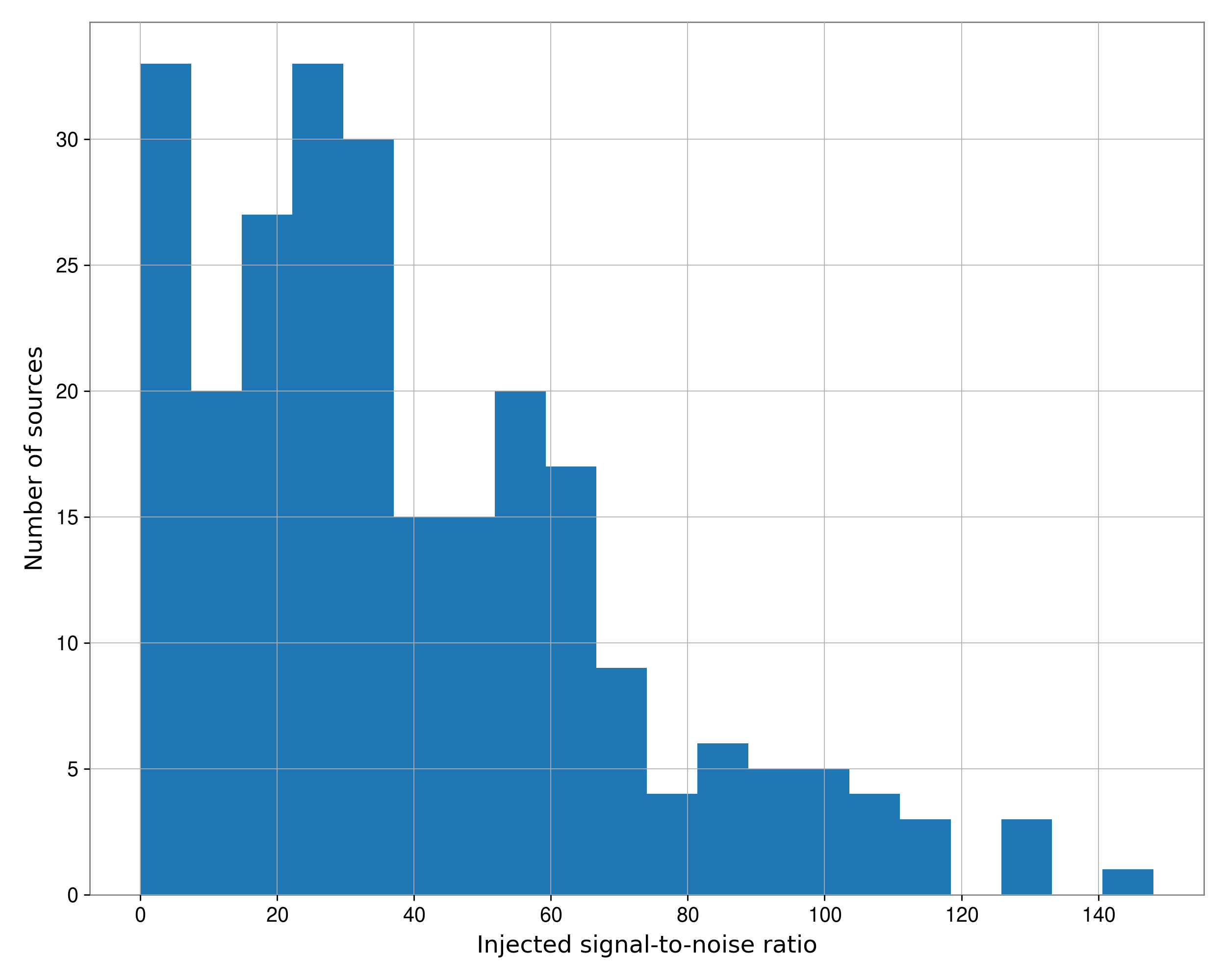
The distributions of signal-to-noise ratios for these simulations is:
Dual harmonic signal#
We produce PP plots for the case of a signal from the \(l=2, m=1,2\) mass quadrupole of a
pulsar, where emission would be at both once and twice the rotation frequency and defined by the
parameters \(C_{12}\), \(C_{22}\), \(\Phi_{12}\), \(\Phi_{22}\), \(\iota\) and
\(\psi\). A Python file to run such an analysis for 250 simulated signals using
KnopePPPlotsDAG is shown below. This also shows the priors used for
the generation of signal parameters and their recovery.
Note
When drawing parameters from the \(C_{12}\) and \(C_{22}\) priors, a maximum cut-off
(maxamp in the code) that is lower than the upper range of the prior is used. This is to
ensure that posteriors are not truncated by the upper end of the prior in this case. However,
this should not bias the recovered credible intervals due to the \(C_{12}\) and
\(C_{22}\) priors being uniform and extending well above the maxamp value.
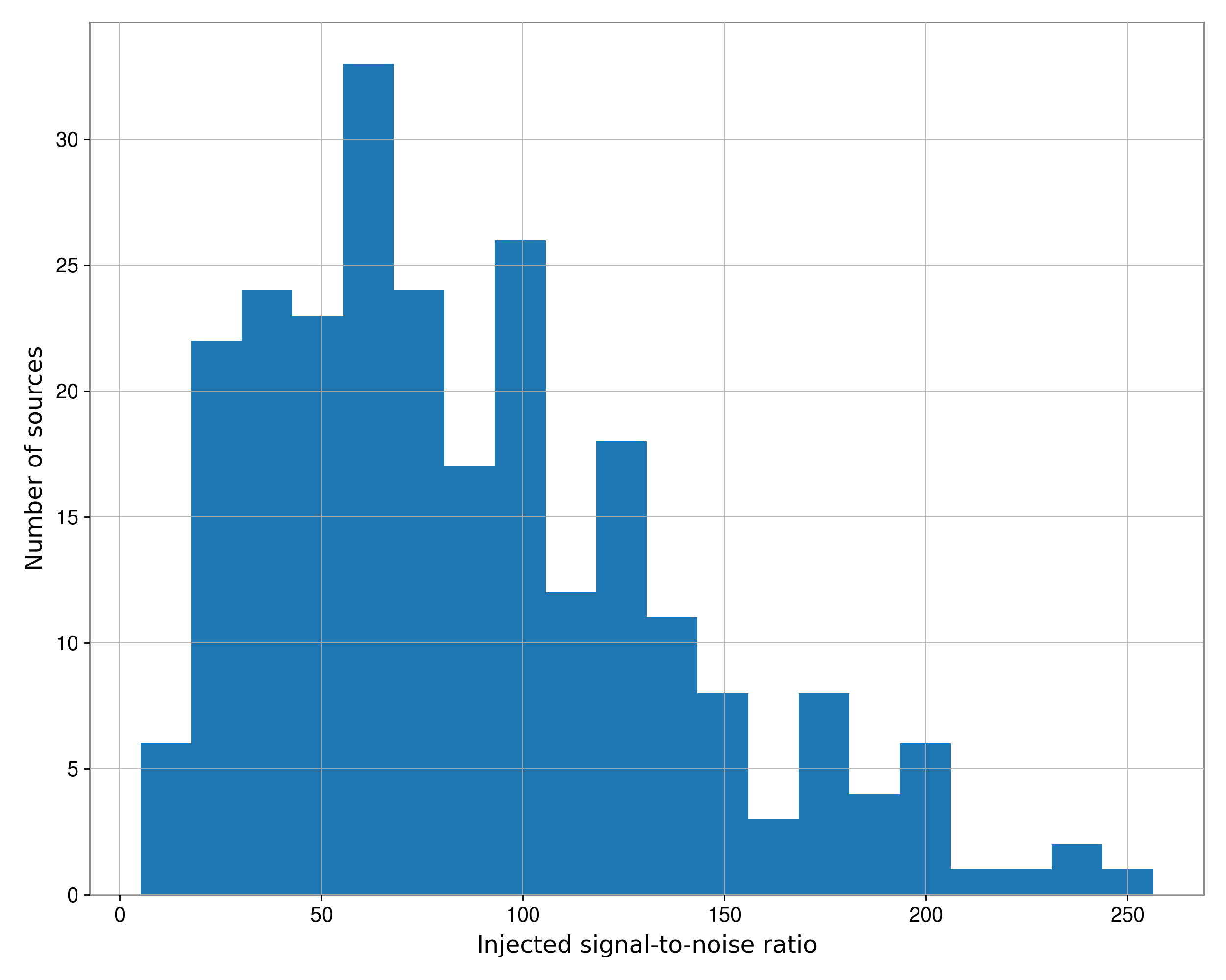
The distributions of signal-to-noise ratios for these simulations is:
#!/usr/bin/env python

"""
Create HTCondor Dag to run a P-P test for the standard four parameters
of a pulsar gravitational-wave signal, assuming emission at twice the rotation
frequency: h0, iota, psi and phi0.
"""

import bilby
import numpy as np

from cwinpy.pe.testing import PEPPPlotsDAG

# set the priors
prior = {}
prior["h0"] = bilby.core.prior.Uniform(minimum=0.0, maximum=1e-22, latex_label="$h_0$")
prior["phi0"] = bilby.core.prior.Uniform(
    name="phi0", minimum=0.0, maximum=np.pi, latex_label=r"$\phi_0$", unit="rad"
)
prior["iota"] = bilby.core.prior.Sine(
    name="iota", minimum=0.0, maximum=np.pi, latex_label=r"$\iota$", unit="rad"
)
prior["psi"] = bilby.core.prior.Uniform(
    name="psi", minimum=0.0, maximum=np.pi / 2, latex_label=r"$\psi$", unit="rad"
)

# Maximum amplitude for any of the injection signal (below the prior maximum)
maxamp = 2.5e-24
det = "H1"  # detector and noise ASD
ninj = 250  # number of simulated signals
basedir = "/home/matthew.pitkin/pptest/fourparameters"  # base directory
accuser = "matthew.pitkin"
accgroup = "aluk.dev.o3.cw.targeted"
sampler = "dynesty"
numba = True
freqrange = (100.0, 200.0)

run = PEPPPlotsDAG(
    prior,
    ninj=ninj,
    maxamp=maxamp,
    detector=det,
    accountuser=accuser,
    accountgroup=accgroup,
    sampler=sampler,
    numba=numba,
    freqrange=freqrange,
    basedir=basedir,
    submit=True,  # submit the DAG
)
#!/usr/bin/env python

"""
Create HTCondor Dag to run a P-P test for the six parameters of a pulsar
gravitational-wave signal, assuming emission at both once and twice the
rotation frequency: c21, c22, iota, psi, phi21, and phi22.
"""

import bilby
import numpy as np

from cwinpy.pe.testing import PEPPPlotsDAG

# set the priors
prior = {}
prior["c21"] = bilby.core.prior.Uniform(
    minimum=0.0, maximum=1e-22, latex_label="$C_{21}$"
)
prior["c22"] = bilby.core.prior.Uniform(
    minimum=0.0, maximum=1e-22, latex_label="$C_{22}$"
)
prior["phi21"] = bilby.core.prior.Uniform(
    name="phi21",
    minimum=0.0,
    maximum=2.0 * np.pi,
    latex_label=r"$\Phi_{21}$",
    unit="rad",
)
prior["phi22"] = bilby.core.prior.Uniform(
    name="phi22",
    minimum=0.0,
    maximum=2.0 * np.pi,
    latex_label=r"$\Phi_{22}$",
    unit="rad",
)
prior["iota"] = bilby.core.prior.Sine(
    name="iota", minimum=0.0, maximum=np.pi, latex_label=r"$\iota$", unit="rad"
)
prior["psi"] = bilby.core.prior.Uniform(
    name="psi", minimum=0.0, maximum=np.pi / 2, latex_label=r"$\psi$", unit="rad"
)

# Maximum amplitude for any of the injection signal (below the prior maximum)
maxamp = 2.5e-24
det = "H1"  # detector and noise ASD
ninj = 250  # number of simulated signals
basedir = "/home/matthew.pitkin/pptest/sixparameters"  # base directory
accuser = "matthew.pitkin"
accgroup = "aluk.dev.o3.cw.targeted"
sampler = "dynesty"
numba = True
freqrange = (100.0, 200.0)


run = PEPPPlotsDAG(
    prior,
    ninj=ninj,
    maxamp=maxamp,
    detector=det,
    accountuser=accuser,
    accountgroup=accgroup,
    sampler=sampler,
    numba=numba,
    freqrange=freqrange,
    basedir=basedir,
    submit=True,  # submit the DAG
)
Pipeline comparison#
We can compare the results of the full pipeline produced by the LALSuite code lalpulsar_knope with that produced using the CWInPy
code cwinpy_knope_pipeline. We will do this comparison by analysing the set of hardware
injections and analysis of real pulsar data using open data from the two LIGO
detectors during the first advanced LIGO observing run (O1).
O1 hardware injections#
To analyse the 15 hardware injections in O1 using the lalpulsar_knope pipeline the following
configuration file (named lalpulsar_knope_O1injections.ini) has been used:
# lalpulsar_knope configuration file for the O1 pulsar hardware injections

[analysis]
ifos = ['H1', 'L1']
starttime = 1126051217
endtime = 1137254417
preprocessing_engine = heterodyne
preprocessing_only = False
postprocessing_only = False
incoherent_only = True
coherent_only = False
freq_factors = [2.0]
ephem_path = /usr/share/lalpulsar
run_dir = /home/matthew/lalapps_knope/O1injections
dag_name = O1injections
submit_dag = True
preprocessing_base_dir = {'H1': '/home/matthew/lalapps_knope/O1injections/H1', 'L1': '/home/matthew/lalapps_knope/O1injections/L1'}
pulsar_param_dir = /home/matthew/miniconda3/envs/cwinpy-dev/lib/python3.8/site-packages/cwinpy/data/O1/hw_inj
log_dir = /home/matthew/lalapps_knope/O1injections/log
injections = True
pickle_file = /home/matthew/lalapps_knope/O1injections/O1injections.pkl
email = matthew.pitkin@ligo.org

[condor]
accounting_group = ligo.dev.o1.cw.targeted.bayesian
accounting_group_user = matthew.pitkin
datafind = /usr/bin/gw_data_find

[datafind]
type = {'H1': 'H1_LOSC_16_V1', 'L1': 'L1_LOSC_16_V1'}
match = localhost

[segmentfind]
server = https://segments.ligo.org
segfind = {'H1': 'H1segments.txt', 'L1': 'L1segments.txt'}

[heterodyne]
universe = vanilla
heterodyne_exec = /usr/bin/lalpulsar_heterodyne
filter_knee = 0.25
coarse_sample_rate = 16384
coarse_resample_rate = 1
coarse_max_data_length = 2048
channels = {'H1': 'H1:GWOSC-16KHZ_R1_STRAIN', 'L1': 'L1:GWOSC-16KHZ_R1_STRAIN'}
fine_resample_rate = 1/60
stddev_thresh = 3.5
binary_output = True
gzip_coarse_output = False
gzip_fine_output = True
coarse_request_memory = 8192
fine_request_memory = 4096

; inputs for running the parameter estimation code lalapps_pulsar_parameter_estimation_nested
[pe]
universe = vanilla
pe_exec = /usr/bin/lalpulsar_parameter_estimation_nested
pe_output_dir = /home/matthew/lalapps_knope/O1injections/nested_samples
prior_options = {'H0': {'priortype': 'uniform', 'ranges': [0., 1e-21]}, 'PHI0': {'priortype': 'uniform', 'ranges': [0., 3.141592653589793]}, 'COSIOTA': {'priortype': 'uniform', 'ranges': [-1.0, 1.0]}, 'PSI': {'priortype': 'uniform', 'ranges': [0.0, 1.5707963267948966]}}
use_parameter_errors = False
n_runs = 2
n_live = 2048
n_mcmc_initial = 0
tolerance = 0.1
non_gr = False
model_type = source
gaussian_like = False
n2p_exec = /usr/bin/lalinference_nest2pos
n2p_output_dir = /home/matthew/lalapps_knope/O1injections/posterior_samples
clean_nest_samples = True
use_gw_phase = False
use_roq = False
pe_request_memory = 4096

; inputs for creating results pages
[results_page]
universe = local
results_exec = /usr/bin/lalapps_knope_result_page.py
collate_exec = /usr/bin/lalapps_knope_collate_results.py
web_dir = /home/matthew/public_html/lalapps_knope/O1injections
base_url = https://results.ligo.uwm.edu/~matthew/lalapps_knope/O1injections
upper_limit = 95
sort_value = name
sort_direction = ascending
results = ['h0ul', 'ell', 'sdrat', 'q22', 'bsn']
parameters = ['f0rot', 'f1rot', 'ra', 'dec', 'dist', 'sdlim']
show_all_posteriors = True
subtract_truths = False
show_priors = True
copy_all_files = False
In this case the included segment lists have been made using the following code:
from cwinpy.heterodyne import generate_segments
from cwinpy.info import HW_INJ_SEGMENTS, RUNTIMES

for det in ["H1", "L1"]:
    start, end = RUNTIMES["O1"][det]
    _ = generate_segments(
        starttime=start,
        endtime=end,
        includeflags=HW_INJ_SEGMENTS["O1"][det]["includesegments"],
        excludeflags=HW_INJ_SEGMENTS["O1"][det]["excludesegments"],
        usegwosc=True,
        writesegments=f"{det}segments.txt",
    )
This has then been submitted (on the UWM Nemo computing cluster) with:
>>> lalpulsar_knope lalpulsar_knope_O1injections.ini
To perform the analysis using CWInPy, the “Quick Setup” has been used:
>>> cwinpy_knope_pipeline --run O1 --hwinj --incoherent-only --output /home/matthew.pitkin/cwinpy_knope/O1injections --accounting-group ligo.dev.o4.cw.targeted.bayesian
Note
Because these analyses used LVK computing resources the
accounting_group / --accounting-group inputs have had to be set.
In terms of wall-clock time
the lalpulsar_knope and cwinpy_knope_pipeline pipelines took 32 hours 8 mins and 13 hours 1
min, respectively (differences here could in part relate to availability of cluster nodes at the
time of running). In terms of total CPU hours used by all the jobs for the lalpulsar_knope and
cwinpy_knope_pipeline pipelines these took approximately 43.4 days and 27.9 days, respectively.
Note
To gather than total time for all the jobs in a Condor DAG I have used:
condor_history matthew -constraint "DAGManJobId == <dagman_id>" -limit <num> -af RemoteWallClockTime | paste -s -d+ - | bc
where <dagman_id> is the ID of the DAGMan job, which can be found in the .dagman.log file.
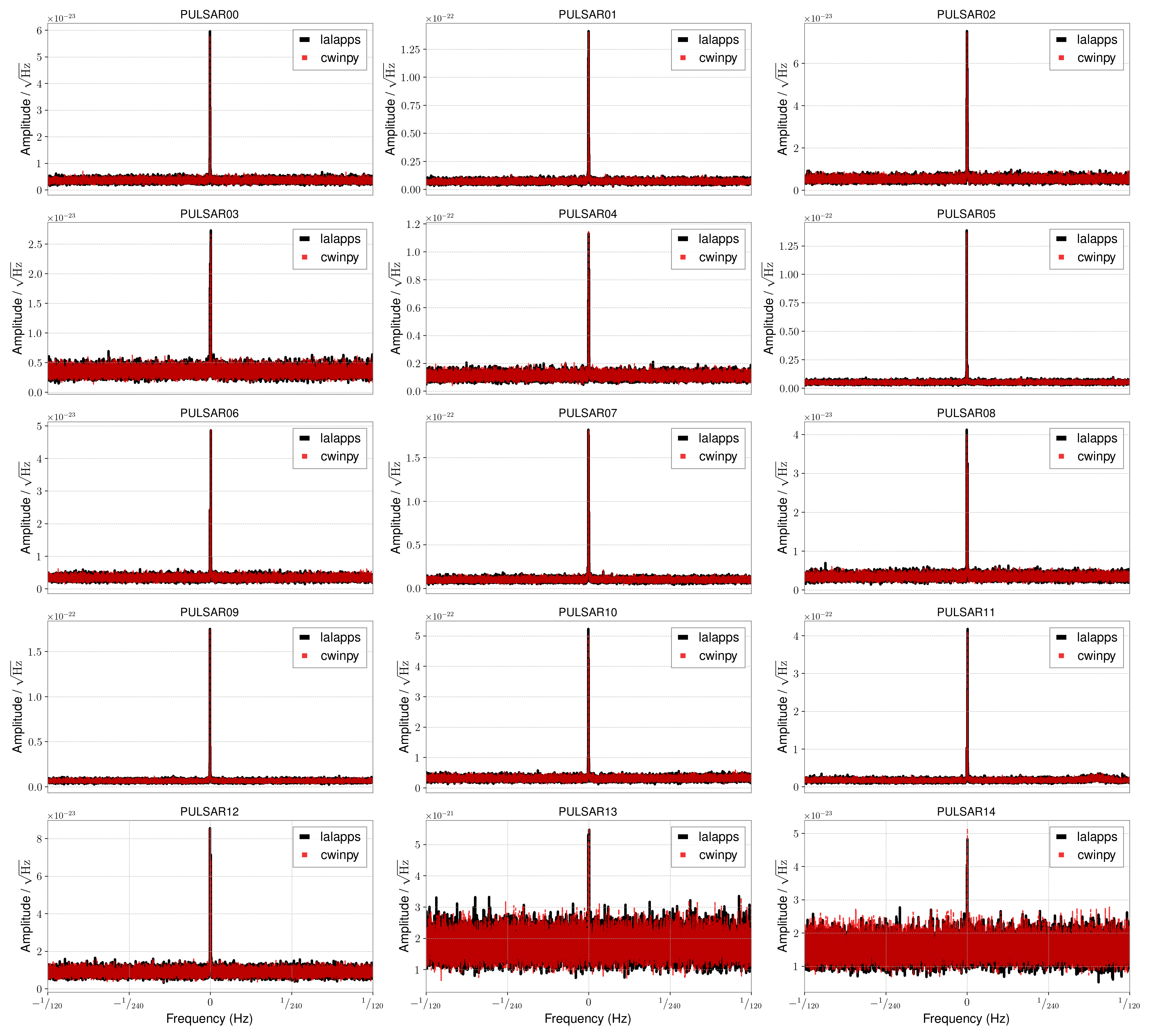
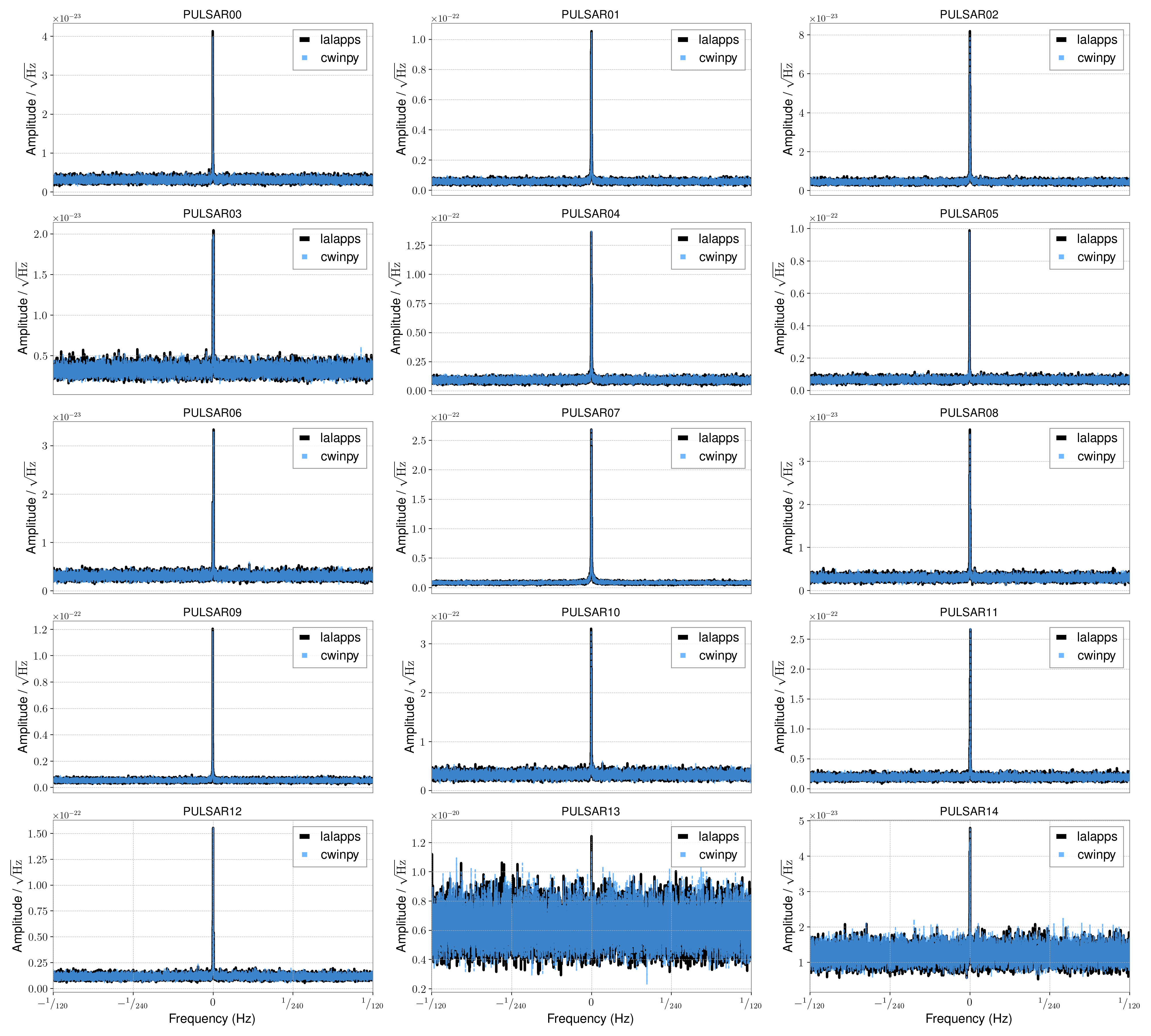
Heterodyned data comparison#
To compare the heterodyned data we can look at the amplitude spectral densities obtained using
lalpulsar_knope and cwinpy_knope_pipeline. The following code has been used to produce these
spectra:
import lal
from cwinpy import HeterodynedData
from matplotlib import pyplot as plt

lalappsbase = "/home/matthew/lalapps_knope/O1injections/{det}/JPULSAR{num}/data/fine/2f/fine-{det}-{span}.txt.gz"
cwinpybase = "/home/matthew/cwinpy_knope/O1injections/{det}/heterodyne_JPULSAR{num}_{det}_2_{span}.hdf5"

numbers = [f"{i:02d}" for i in range(15)]

timespans = {
    "lalapps": {"H1": "1126051217-1137254417", "L1": "1126051217-1137254417"},
    "cwinpy": {"H1": "1129136736-1137253524", "L1": "1126164689-1137250767"},
}

for det in ["H1", "L1"]:
    fig, axs = plt.subplots(5, 3, figsize=(20, 18))

    # loop over pulsars
    for num, ax in zip(numbers, axs.flat):
        # read in heterodyned data
        ck = HeterodynedData(cwinpybase.format(det=det, num=num, span=timespans["cwinpy"][det]))
        lk = HeterodynedData(lalappsbase.format(det=det, num=num, span=timespans["lalapps"][det]))

        # plot median amplitude spectral densities of data
        lk.power_spectrum(remove_outliers=True, dt=int(lal.DAYSID_SI * 10), asd=True, label="lalapps", lw=3, color="k", ax=ax)
        ck.power_spectrum(remove_outliers=True, dt=int(lal.DAYSID_SI * 10), asd=True, label="cwinpy", alpha=0.8, ls="--", ax=ax)
        ax.set_title(f"PULSAR{num}")

        if int(num) < 12:
            ax.xaxis.set_visible(False)

    fig.tight_layout()
    fig.savefig(f"hwinj_comparison_spectrum_{det}.png", dpi=200)
giving the following spectra for H1:
and L1:
Injection parameter comparison#
To compare the final parameter estimation between the lalpulsar_knope and
cwinpy_knope_pipeline to following code has been used:
import os
from cwinpy.plot import Plot
from cwinpy.info import HW_INJ
from gwpy.plot.colors import GW_OBSERVATORY_COLORS

basedir = "/home/matthew"

cwinpydir = os.path.join(basedir, "cwinpy_knope", "O1injections", "results")
lppndir = os.path.join(basedir, "lalapps_knope", "O1injections", "posterior_samples")

for pulnum in range(15):
    pulsar = f"JPULSAR{pulnum:02d}"

    for det in ["H1", "L1"]:
        results = {}
        colors = {}

        for a in ["cwinpy", "lalapps"]:
            if a == "cwinpy":
                resfile = os.path.join(cwinpydir, pulsar, f"cwinpy_pe_{det}_{pulsar}_result.hdf5")
                colors[a] = GW_OBSERVATORY_COLORS[det]
            else:
                resfile = os.path.join(lppndir, pulsar, det, "2f", f"posterior_samples_{pulsar}.hdf")
                colors[a] = "grey"
            results[a] = resfile

        p = Plot(
            results,
            parameters=["h0", "iota", "phi0", "psi"],
            plottype="corner",
            pulsar=HW_INJ["O1"]["hw_inj_files"][pulnum],
            untrig="cosiota"
        )

        fig = p.plot(colors=colors)
        p.fig.suptitle(f"{det}: {pulsar}")
        p.save(f"{pulsar}_{det}_plot.png", dpi=200)

        fig.clf()
        fig.close()
which produces the following plots:
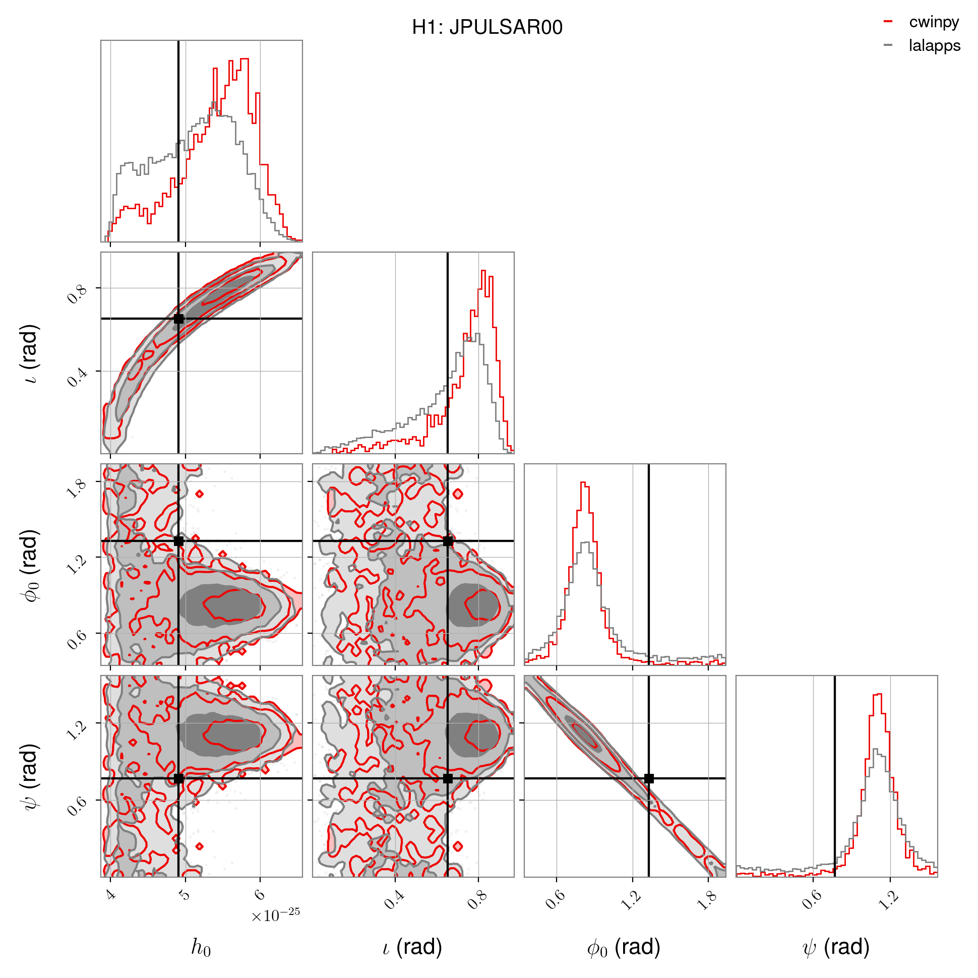
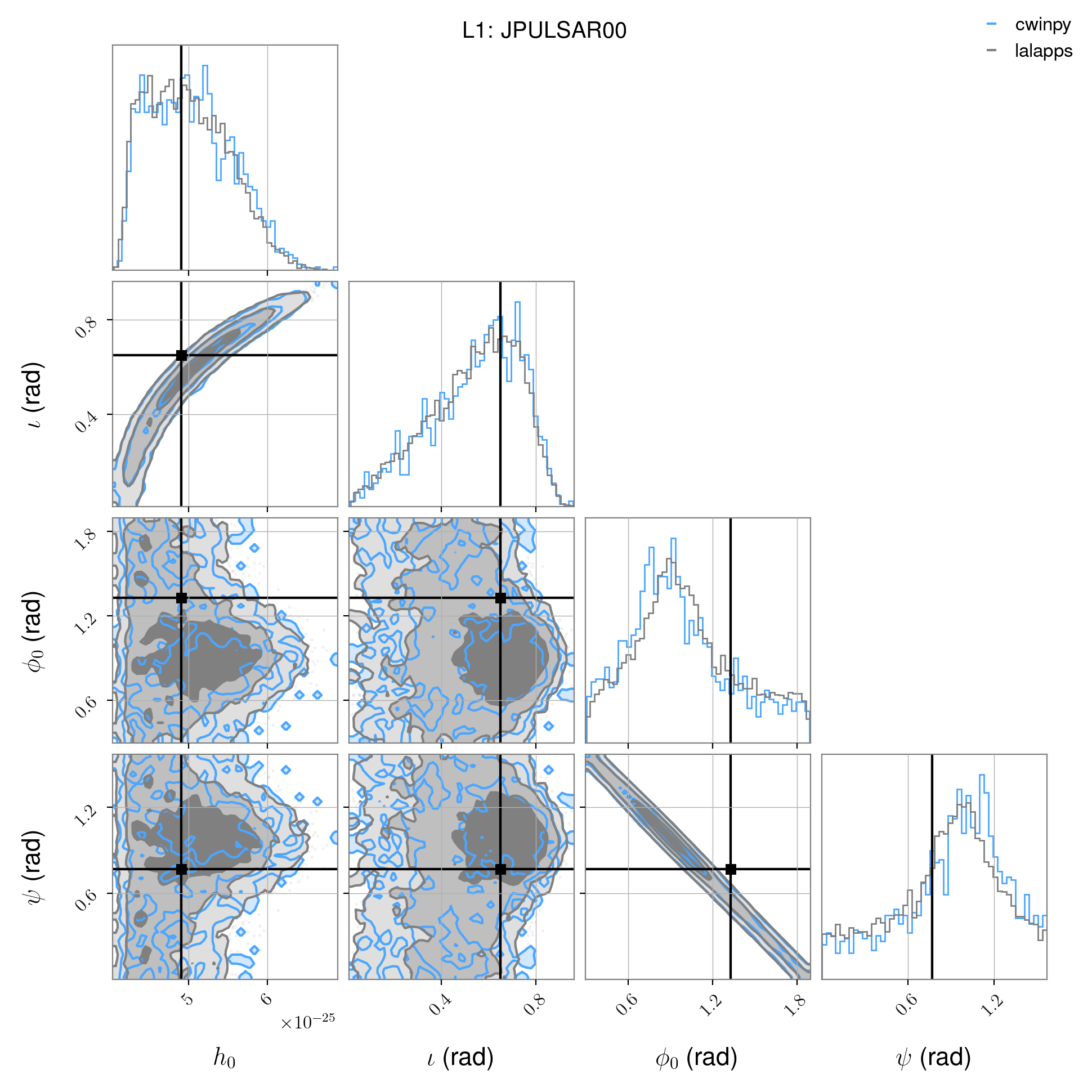
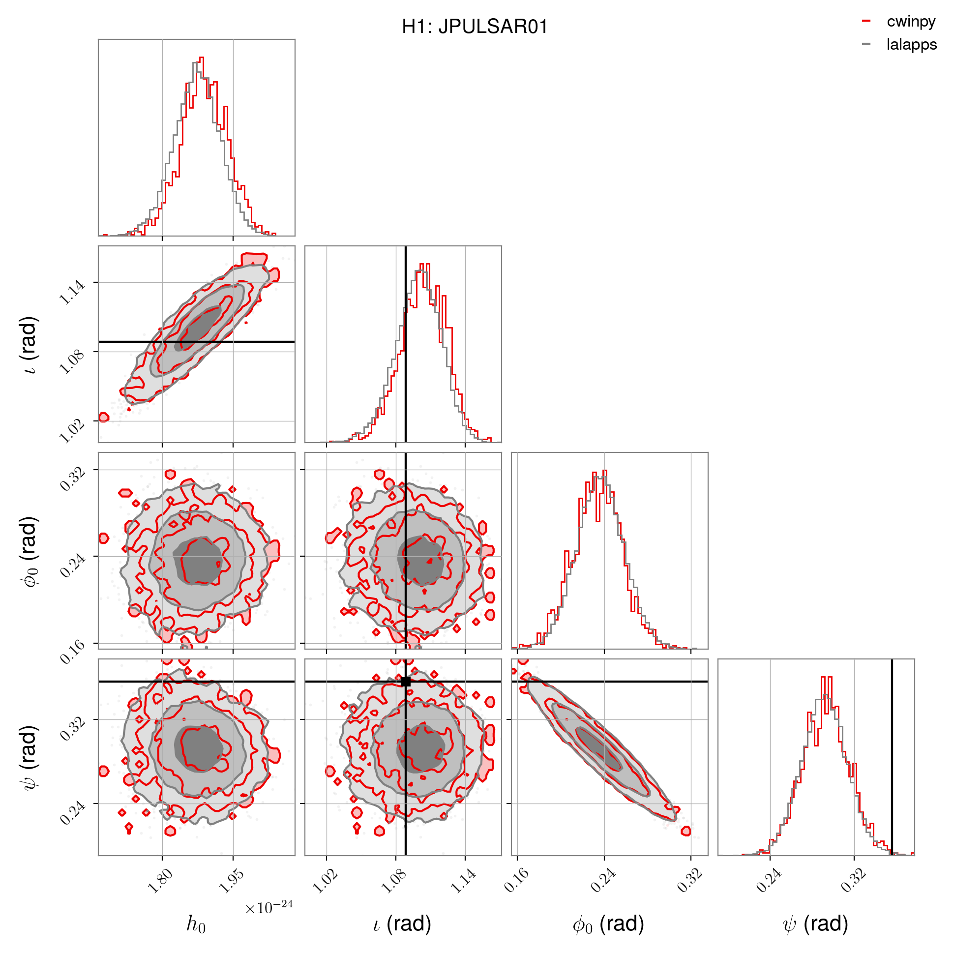
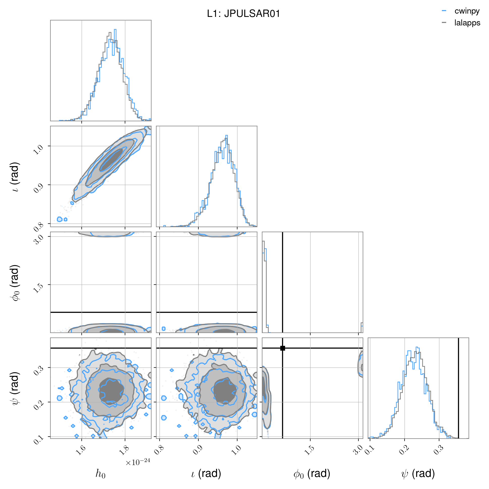
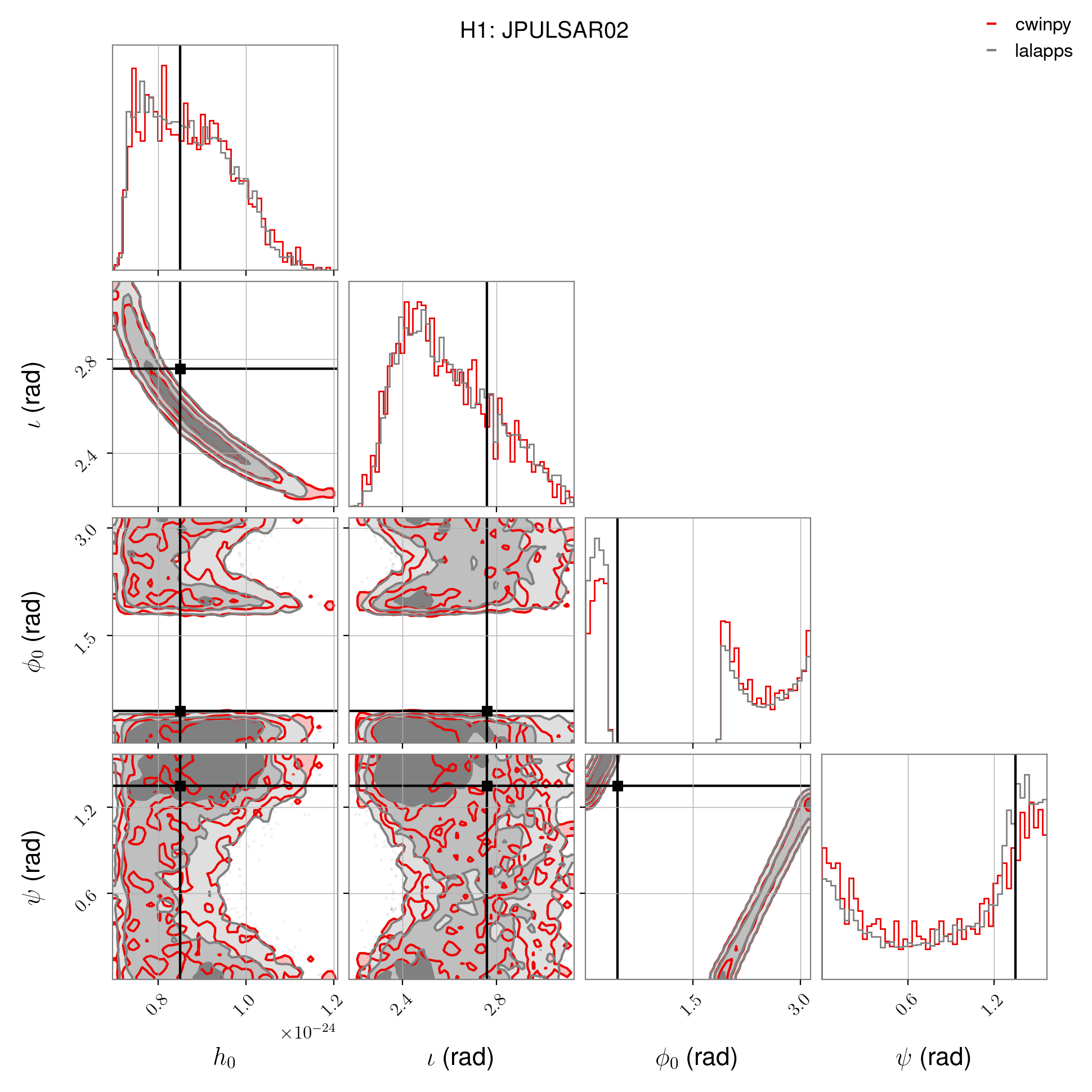
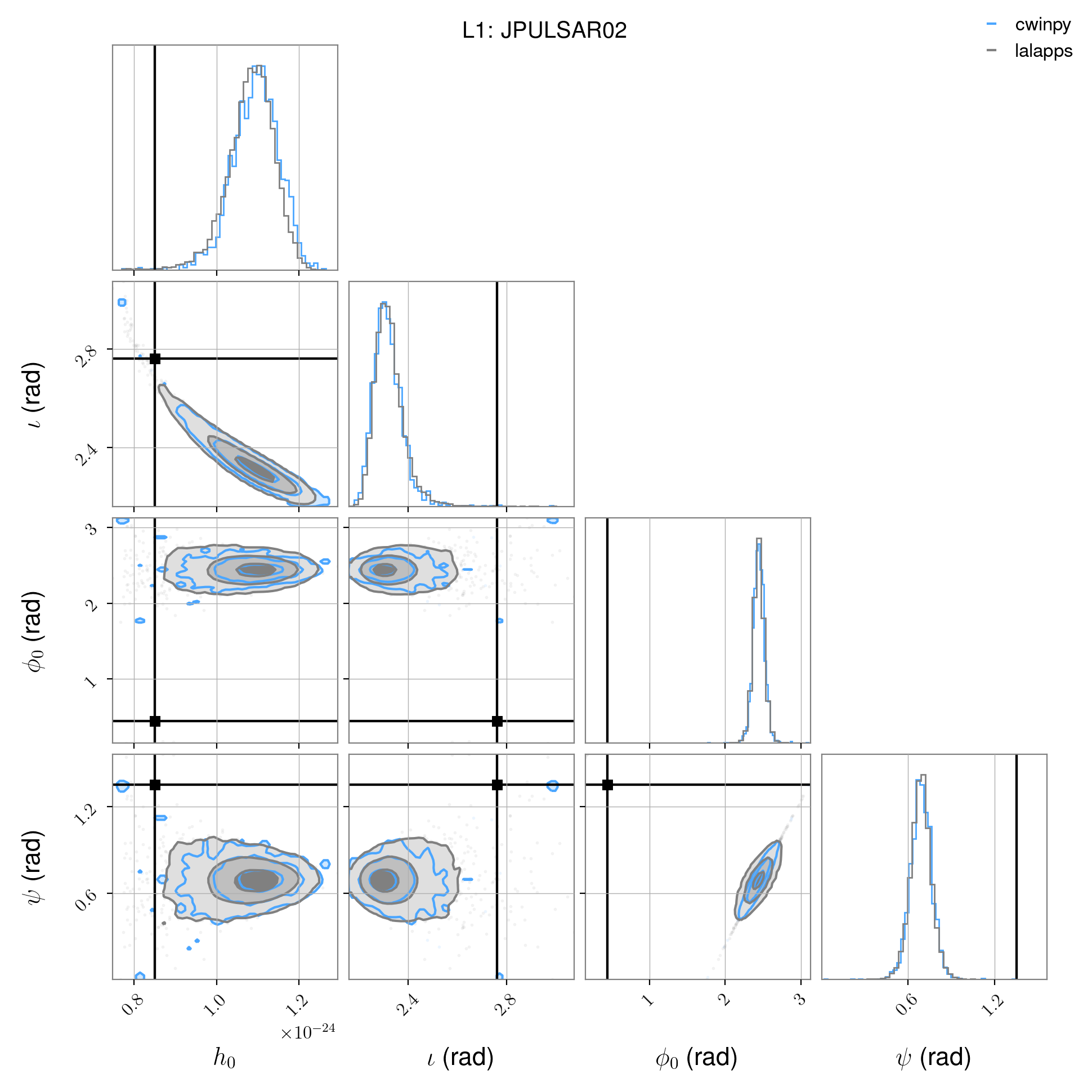
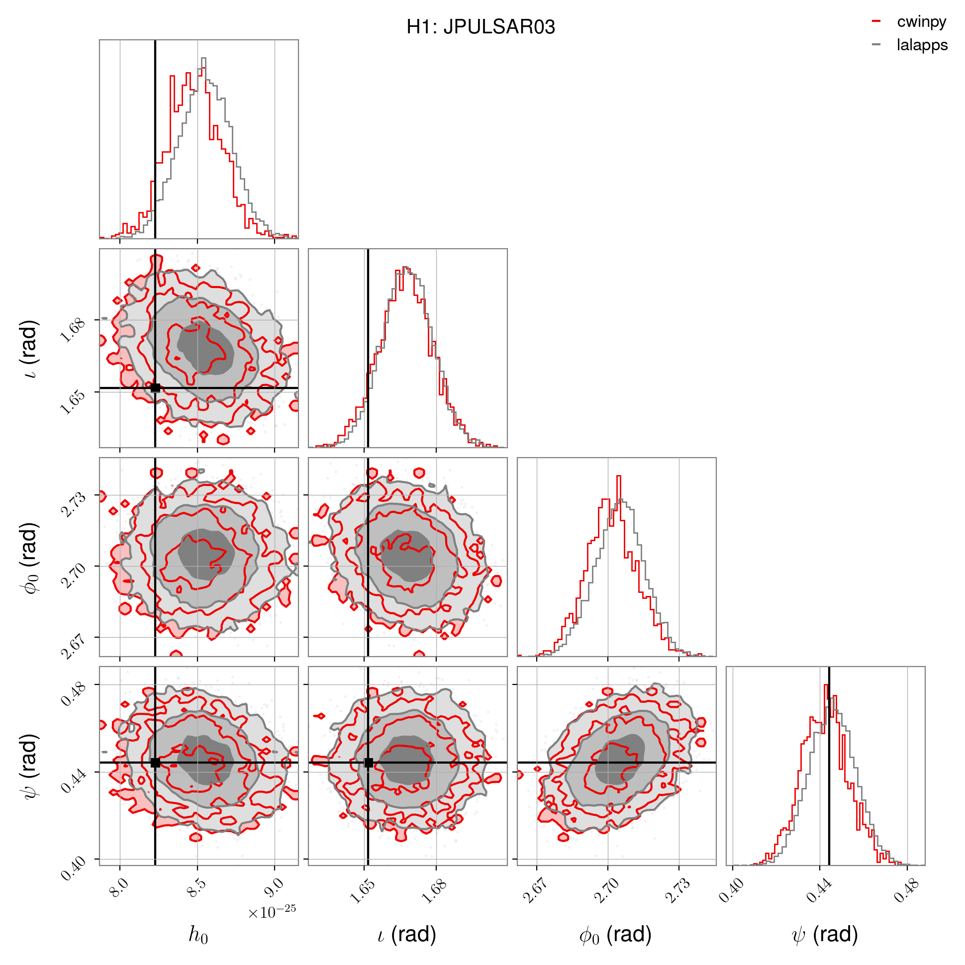
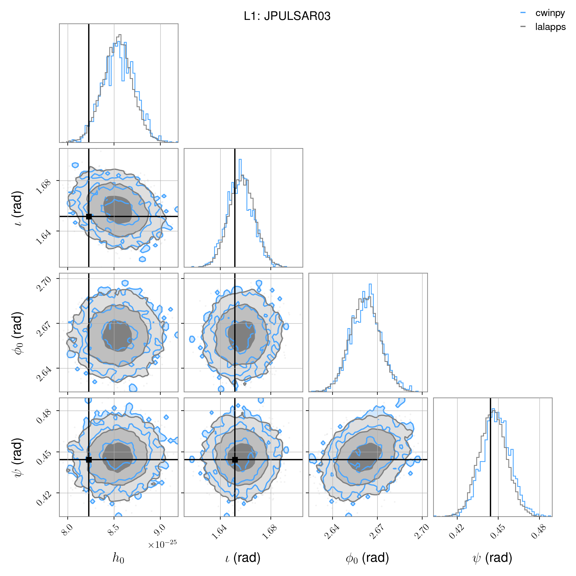
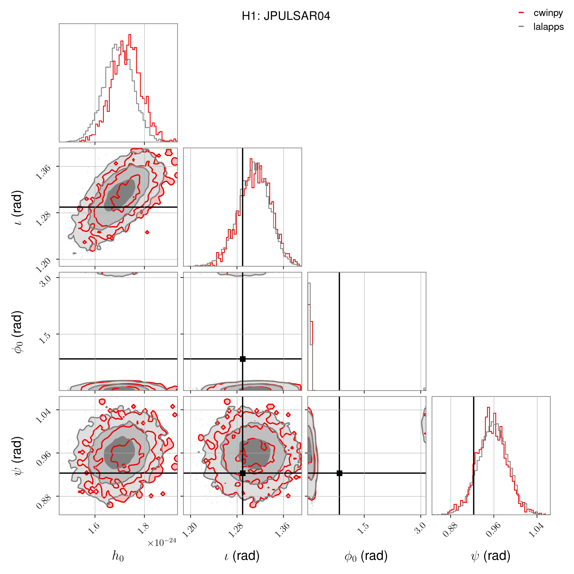
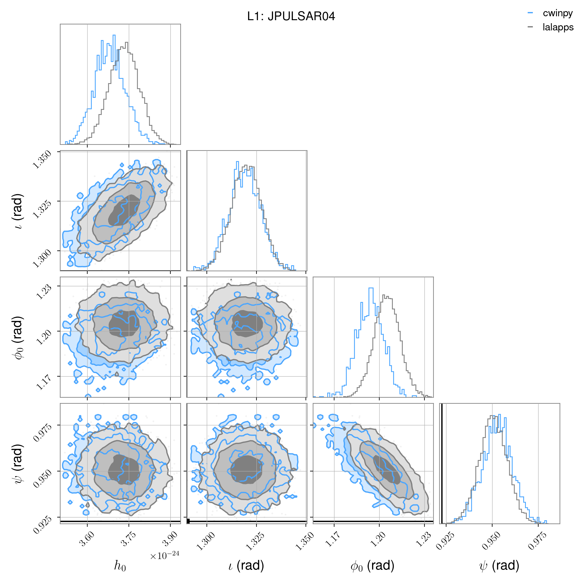
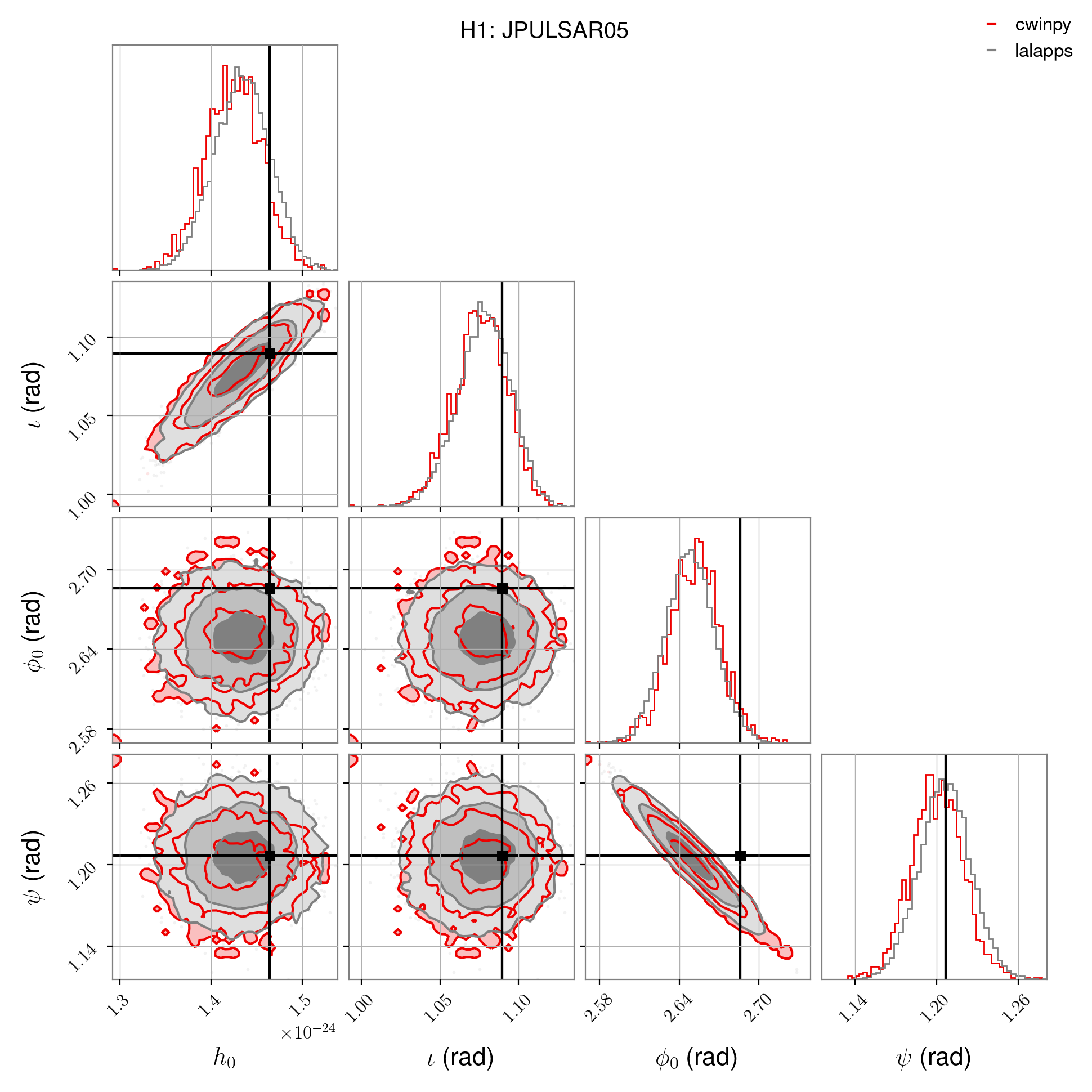
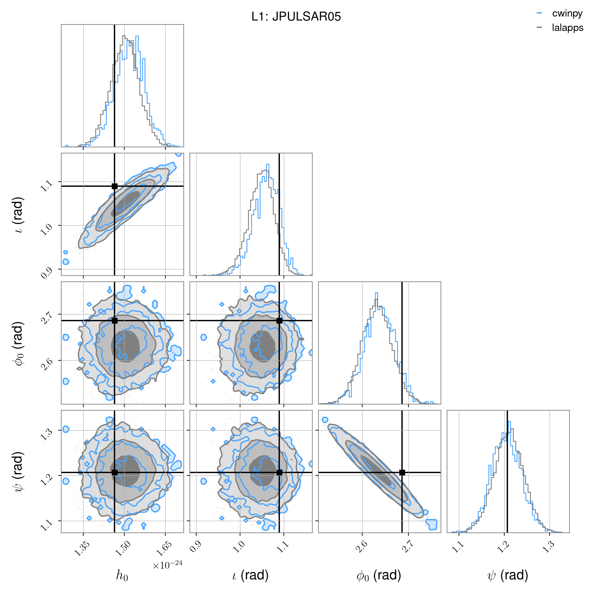
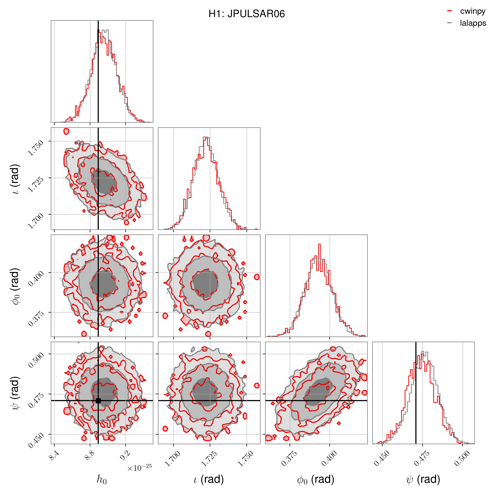
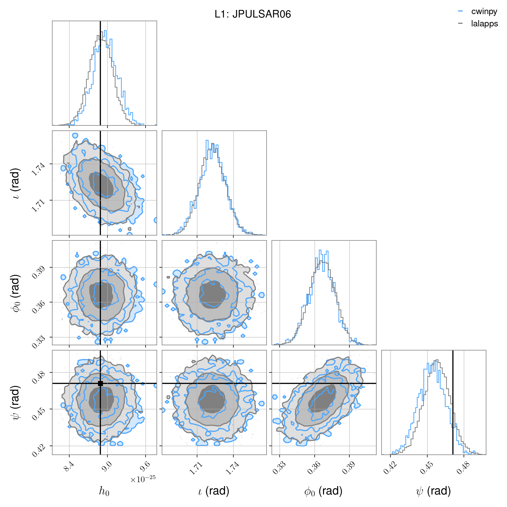
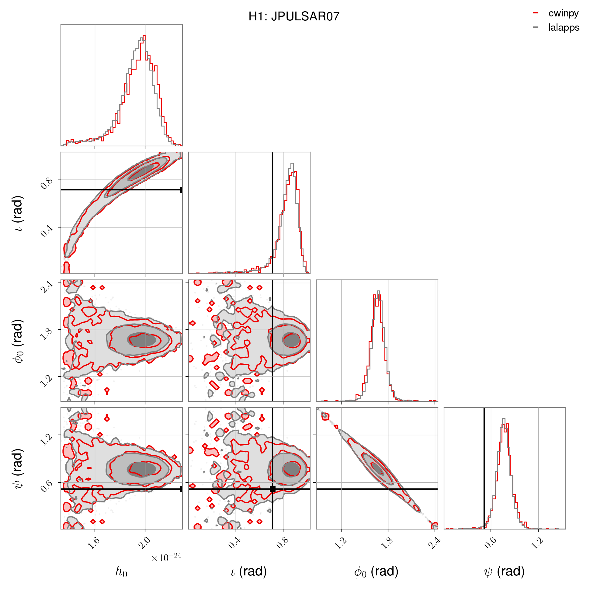
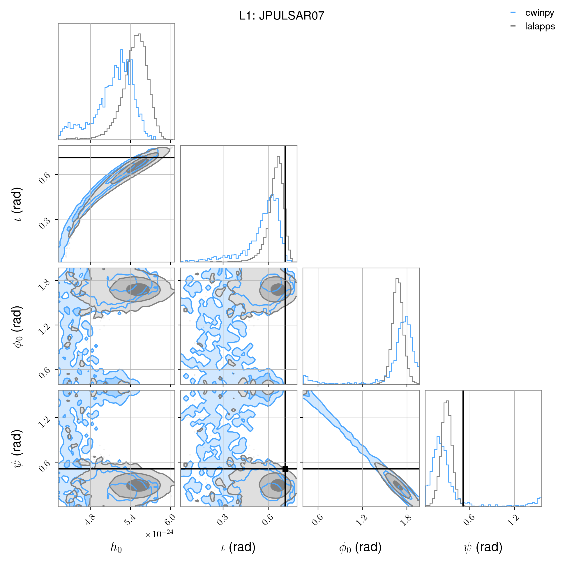
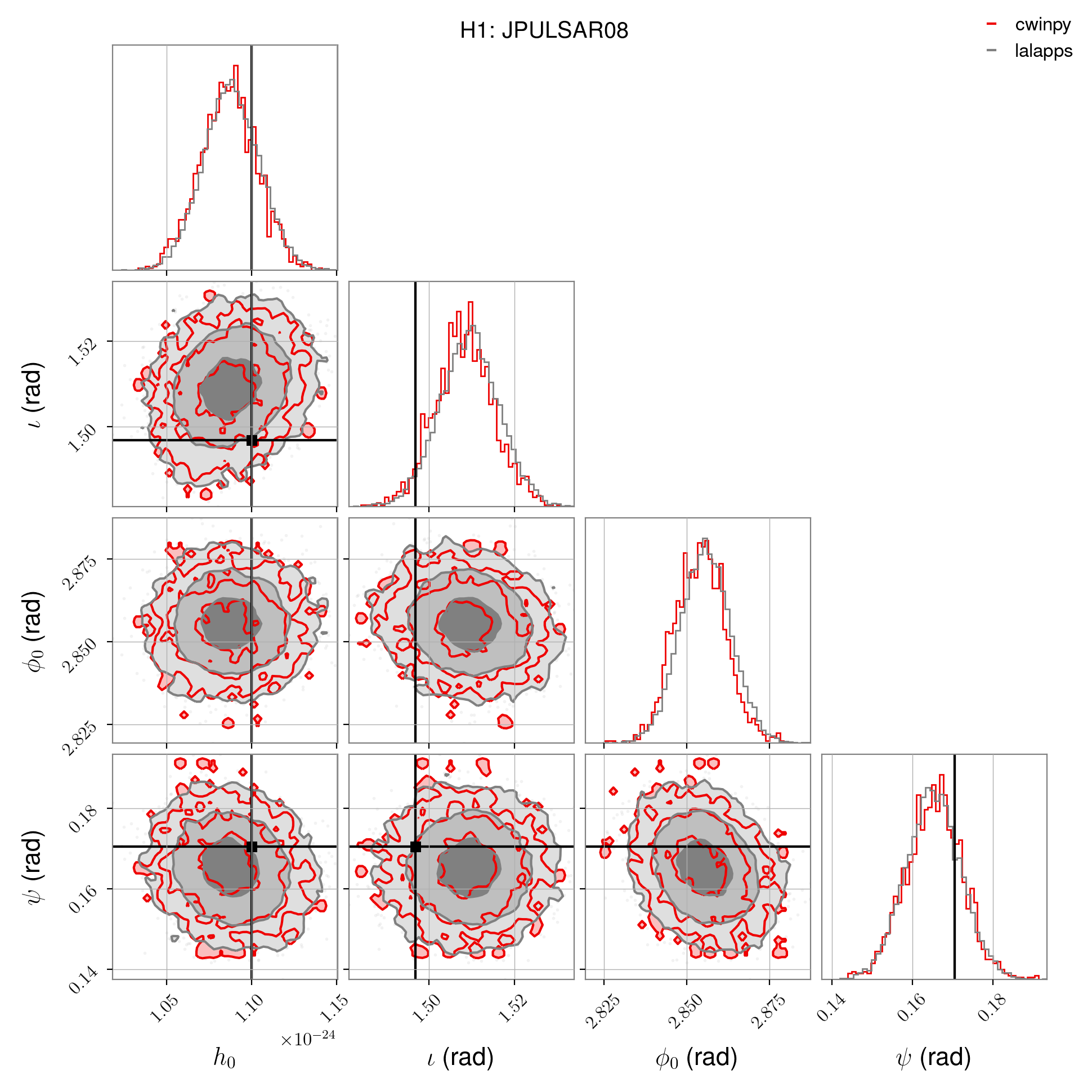
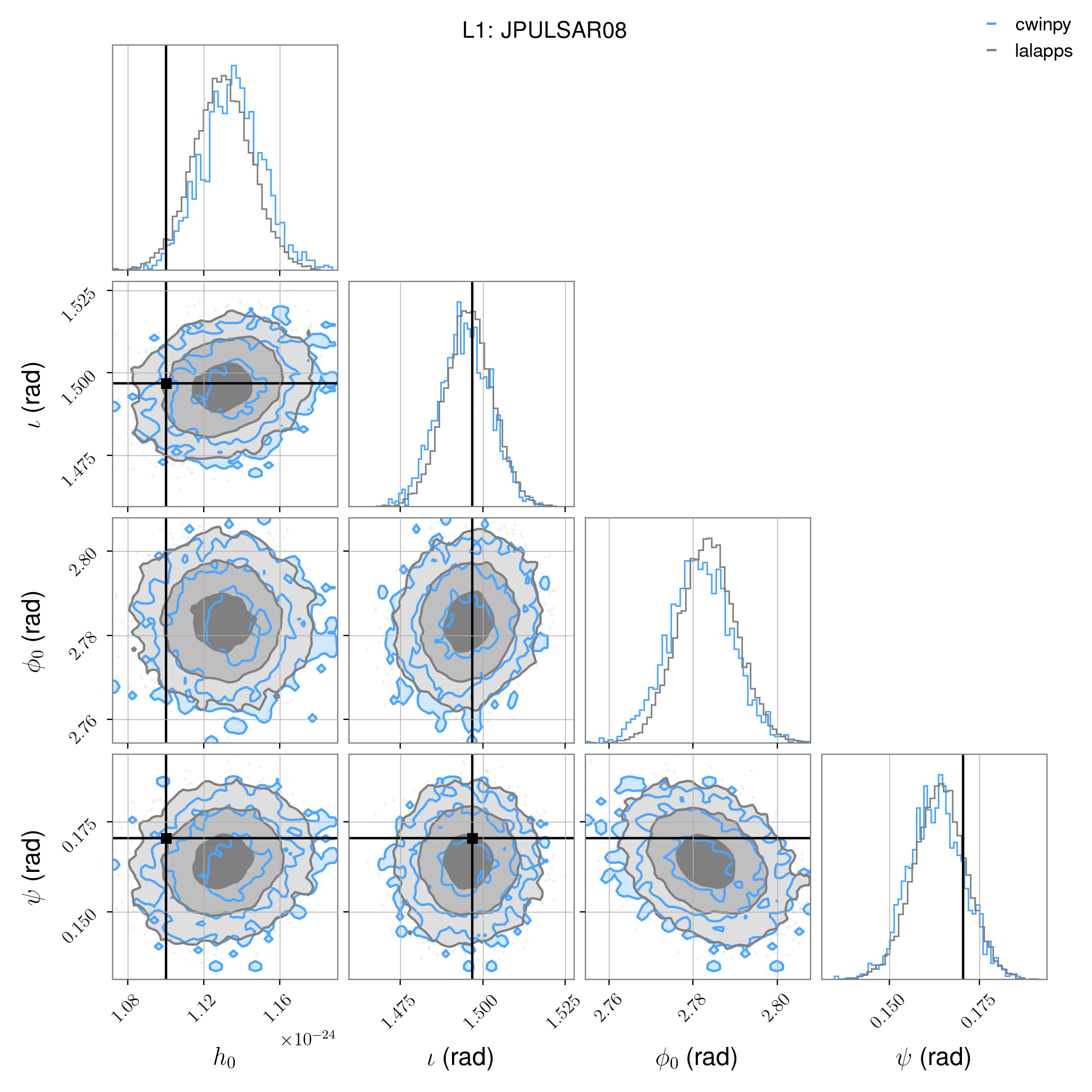
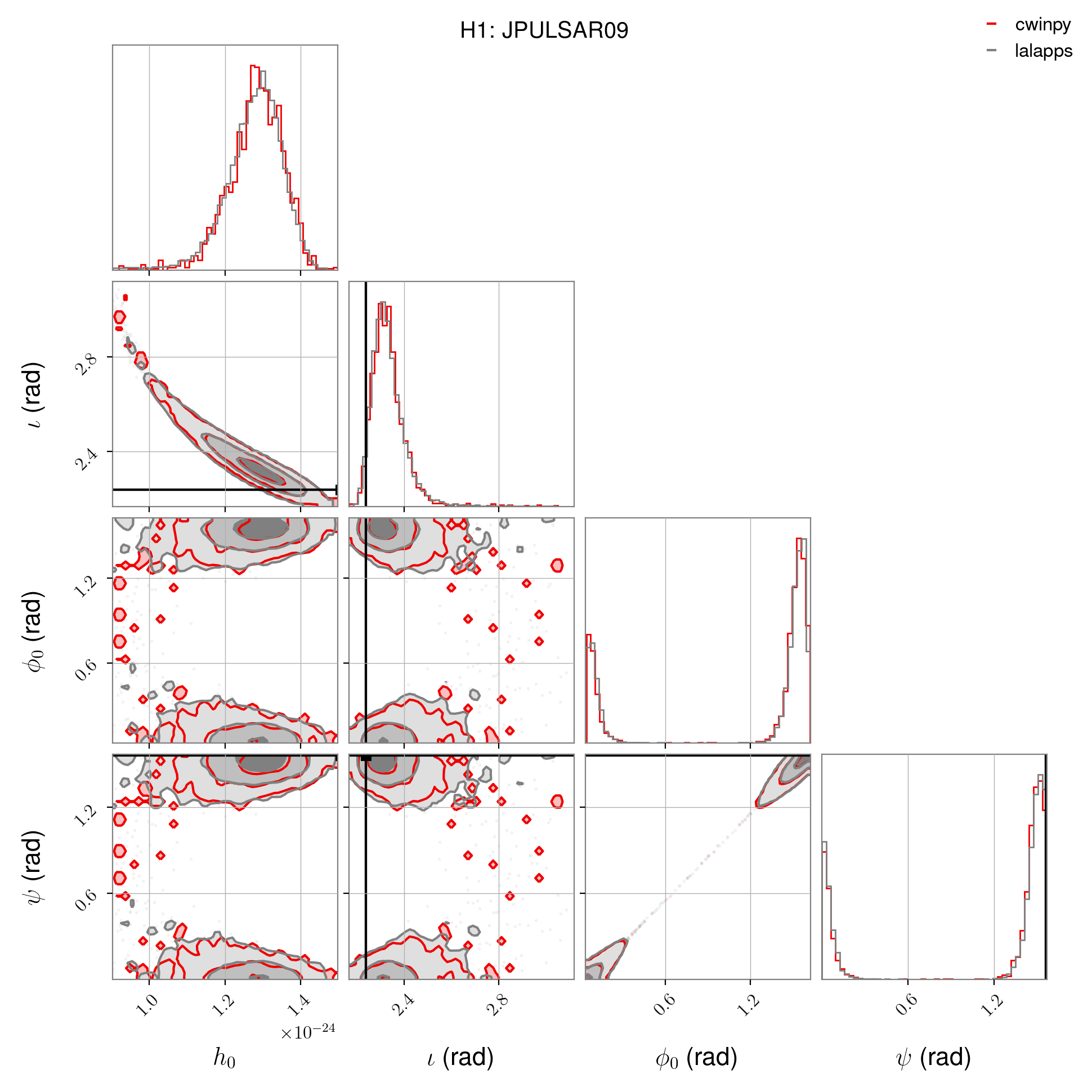
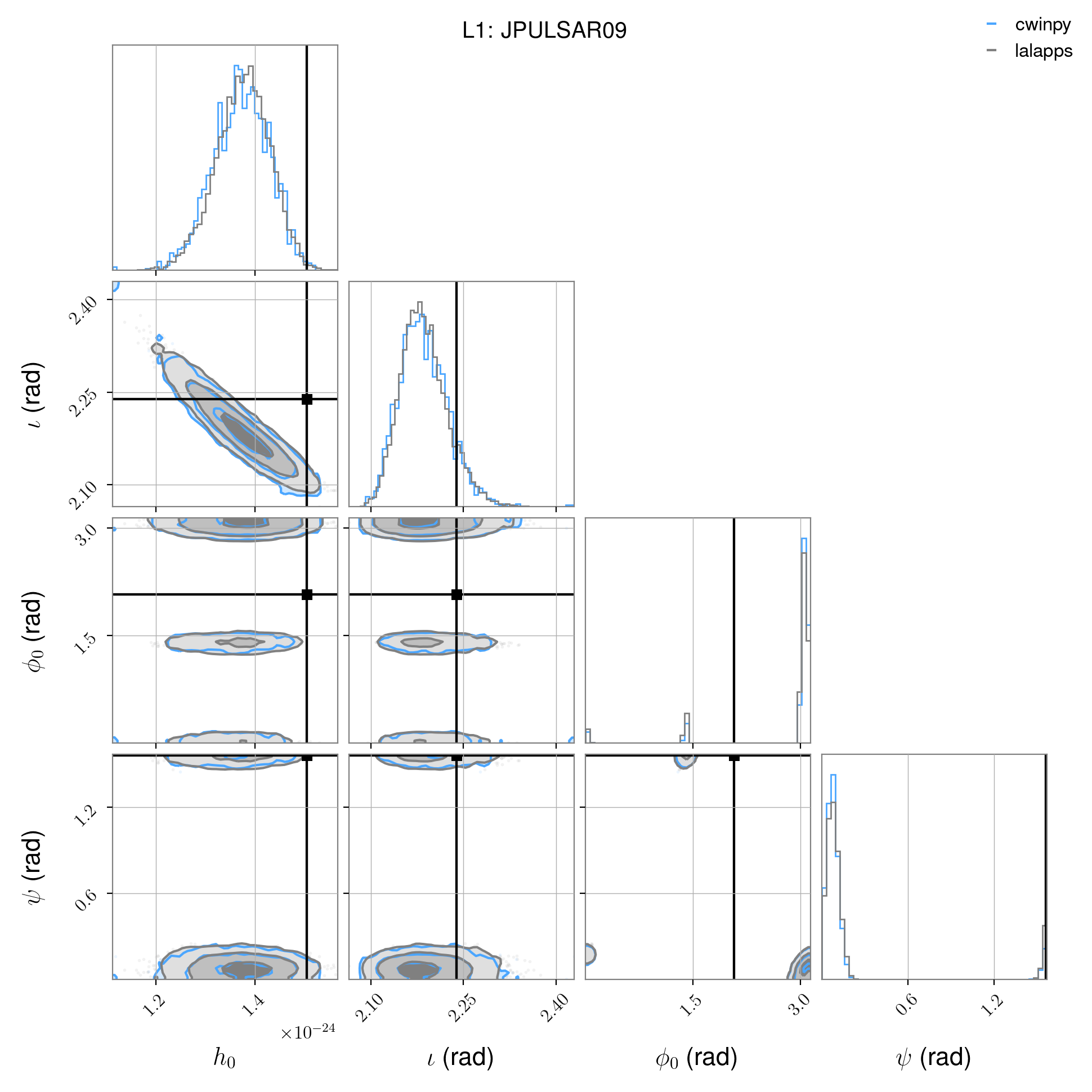
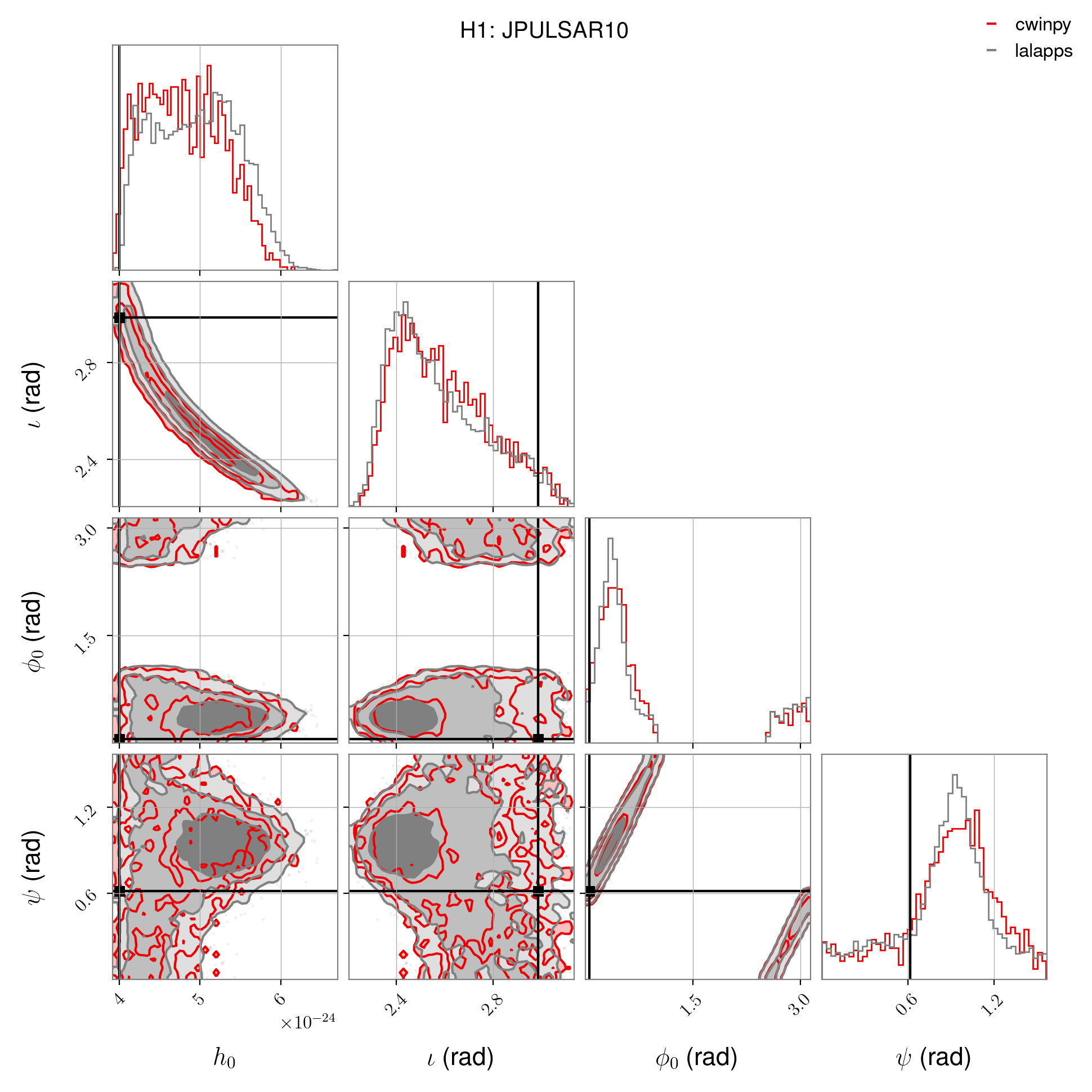
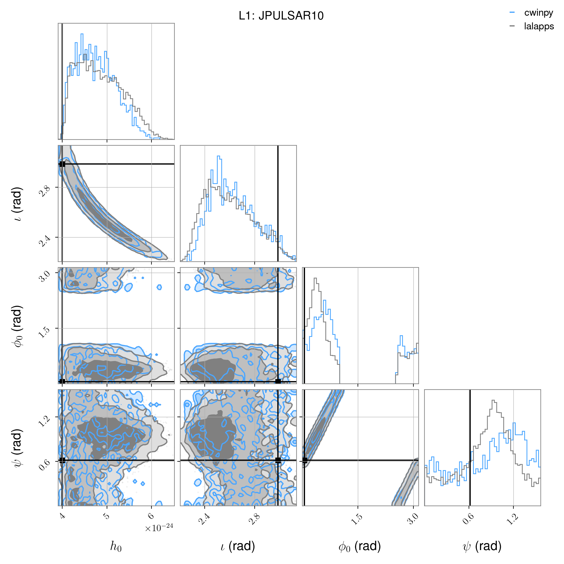
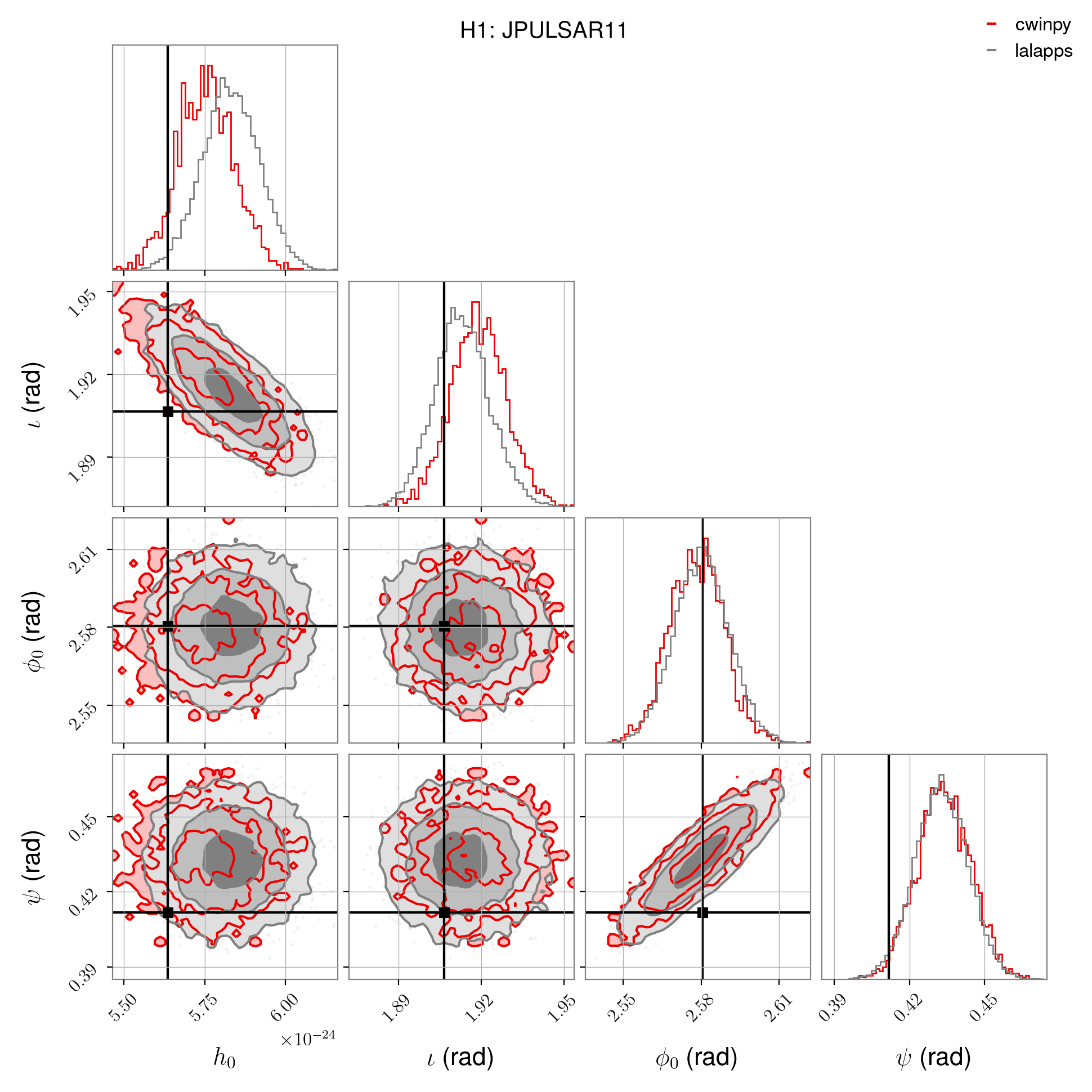
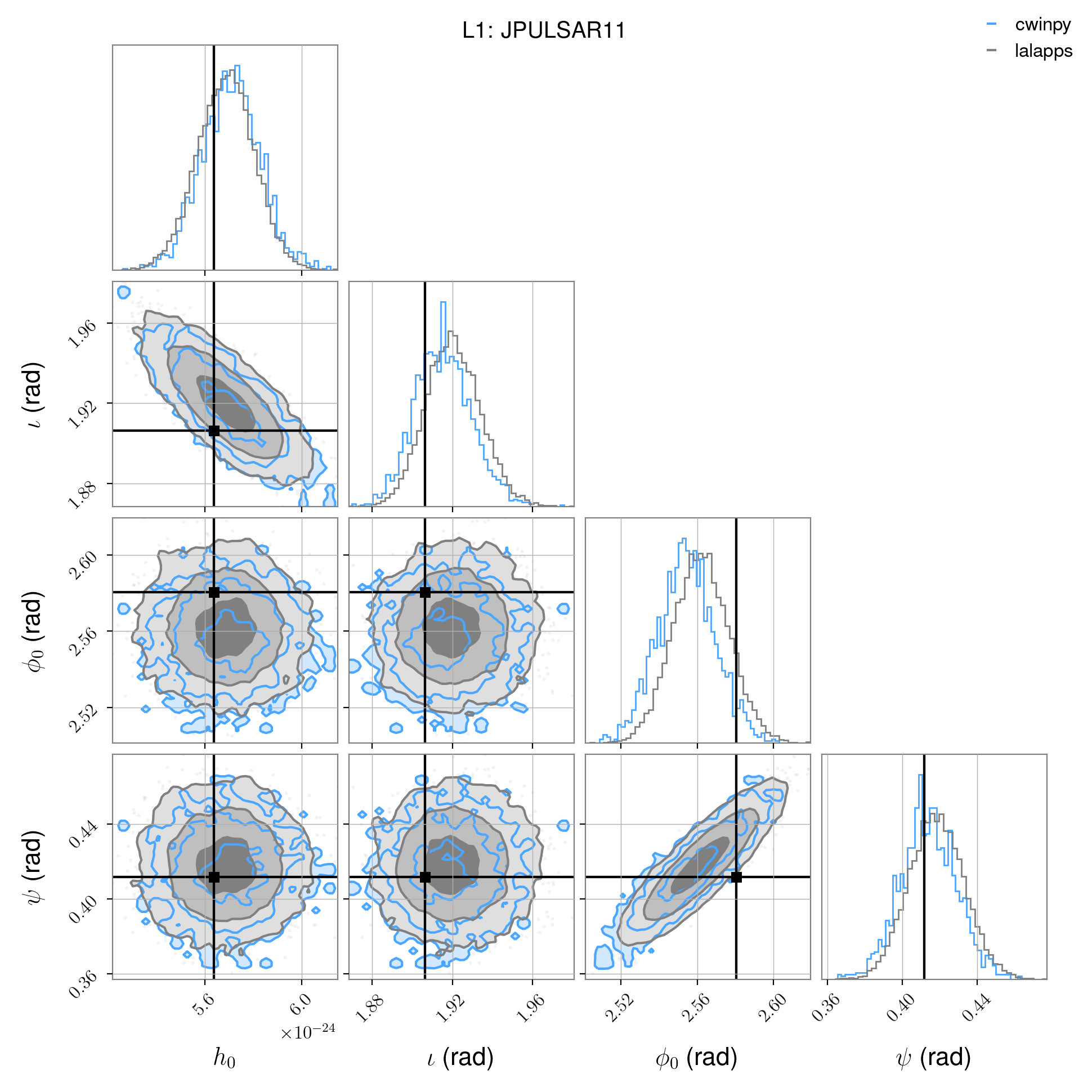
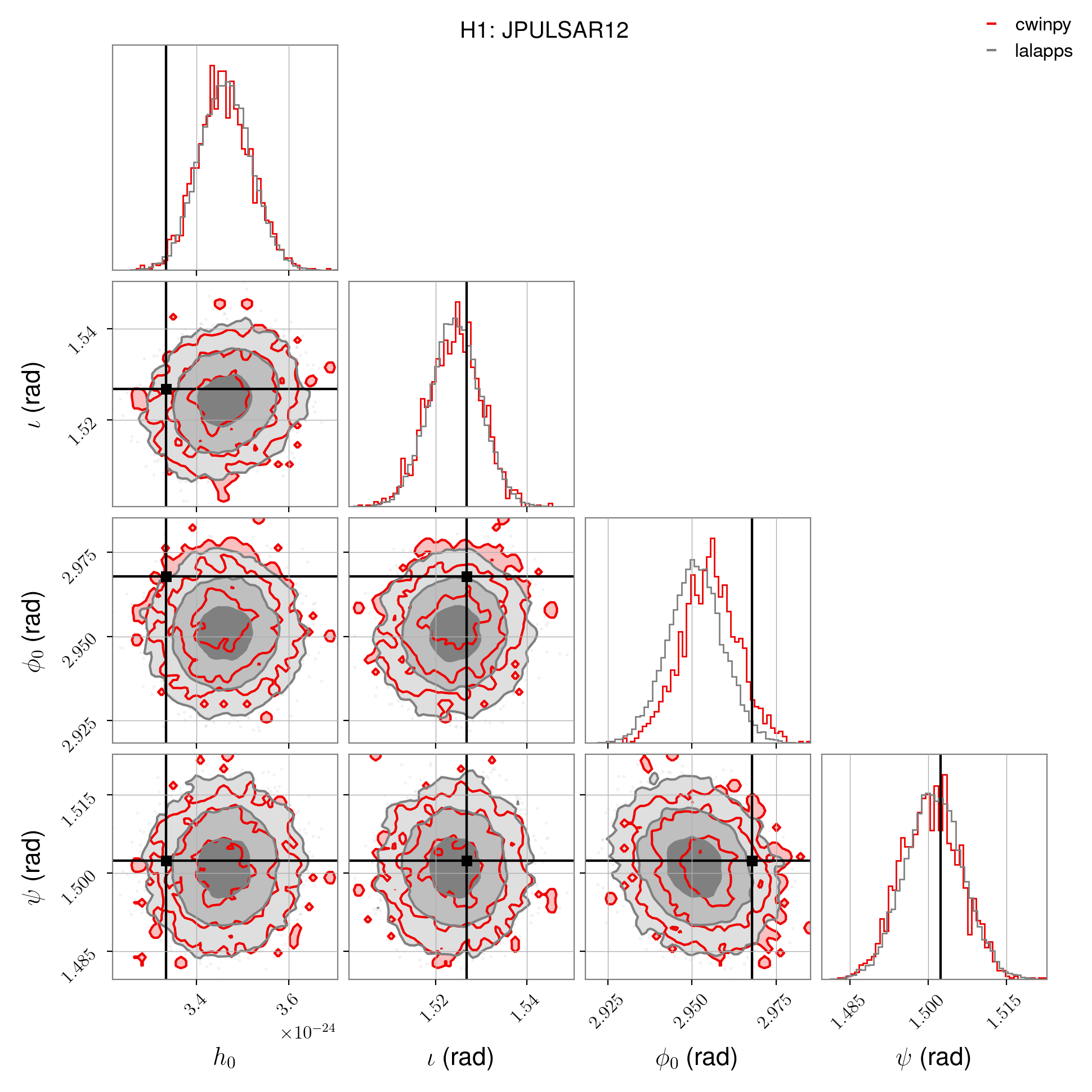
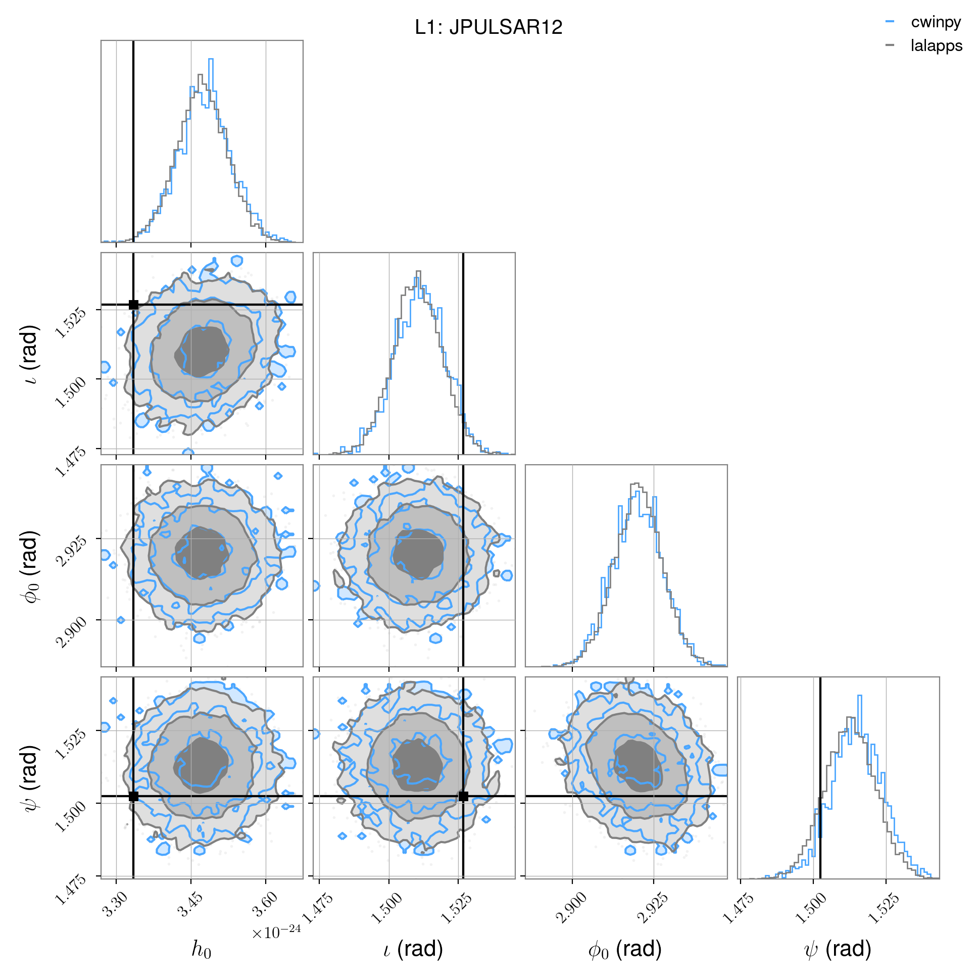
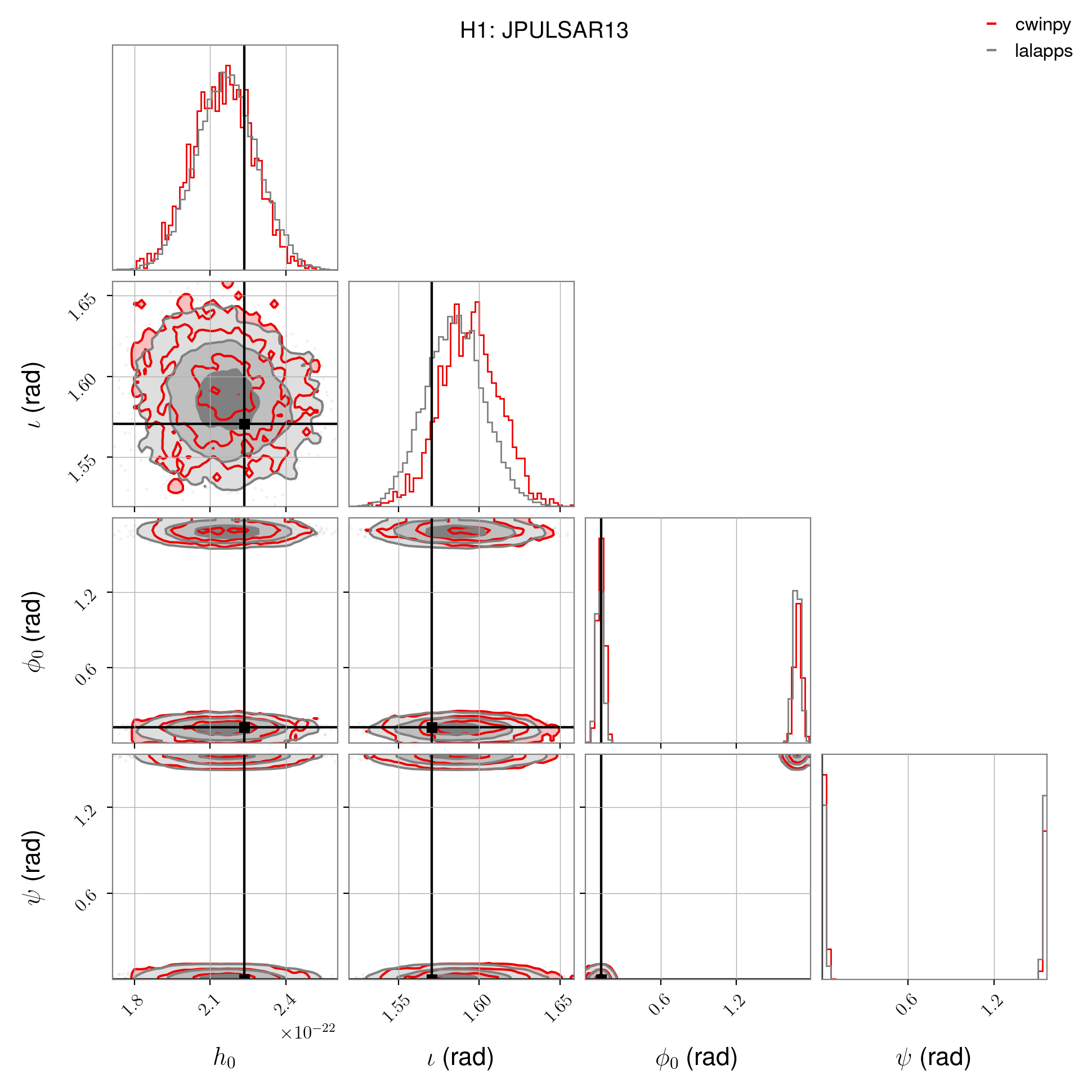
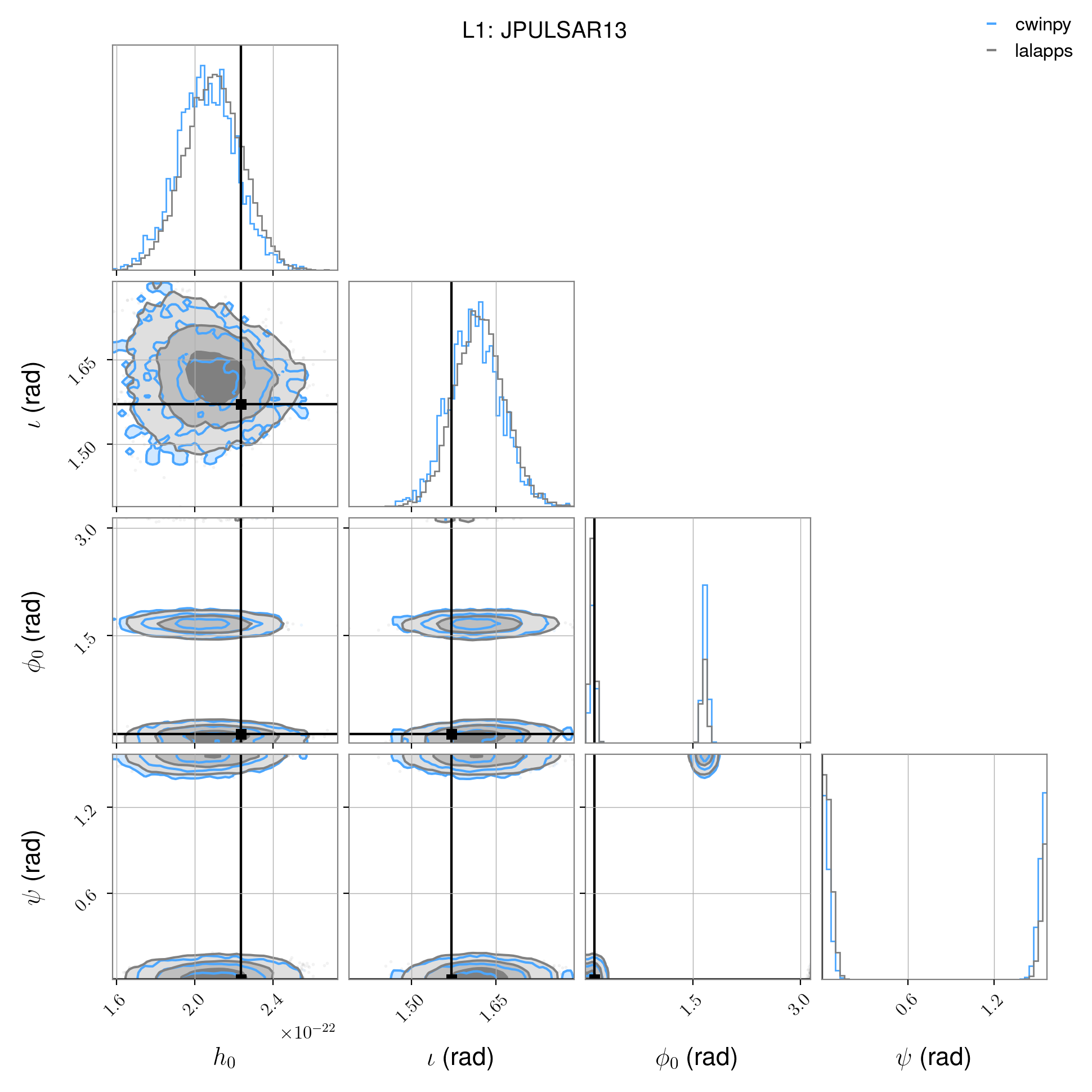
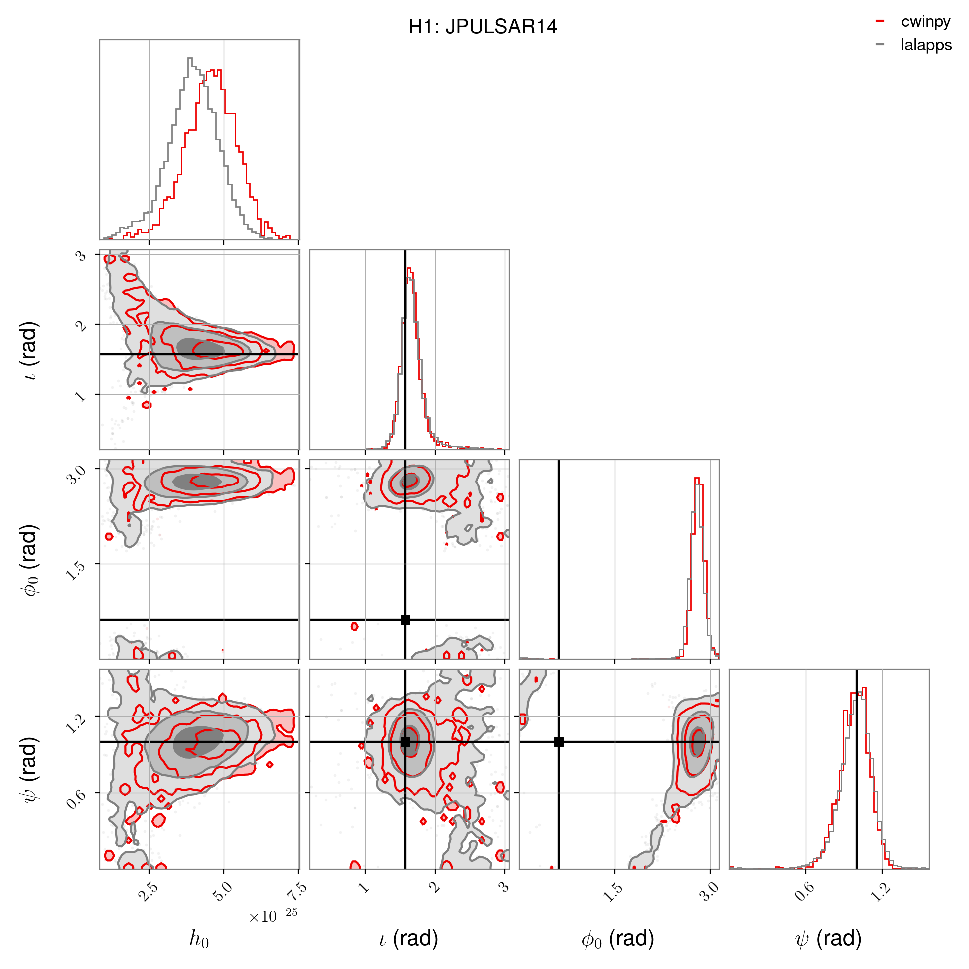
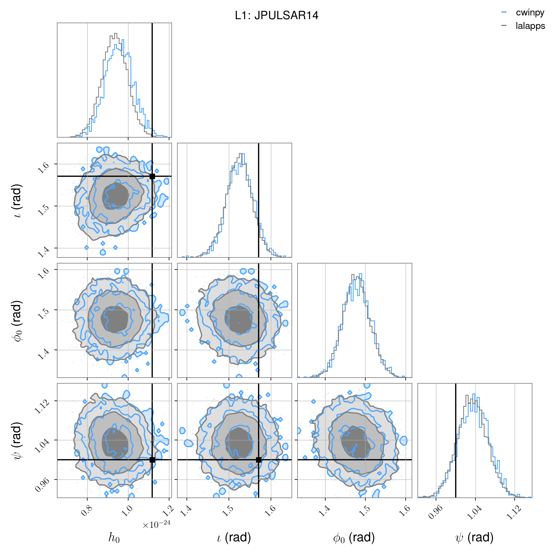
These show very consistent posteriors produced by both codes, which extract the parameters as
expected. They would not be expected to be identical due to a range of differences including:
lalpulsar_knope performed the heterodyne in two stages rather than the one used by
cwinpy_knope_pipeline; lalpulsar_knope uses a low-pass filter with knee frequency of 0.25 Hz
rather than the default 0.1 Hz used by cwinpy_knope_pipeline; the outlier vetoing for the two
codes is different; the default “chunking” of the heterodyned data into stationary segments used
during parameter estimation is different between the codes.