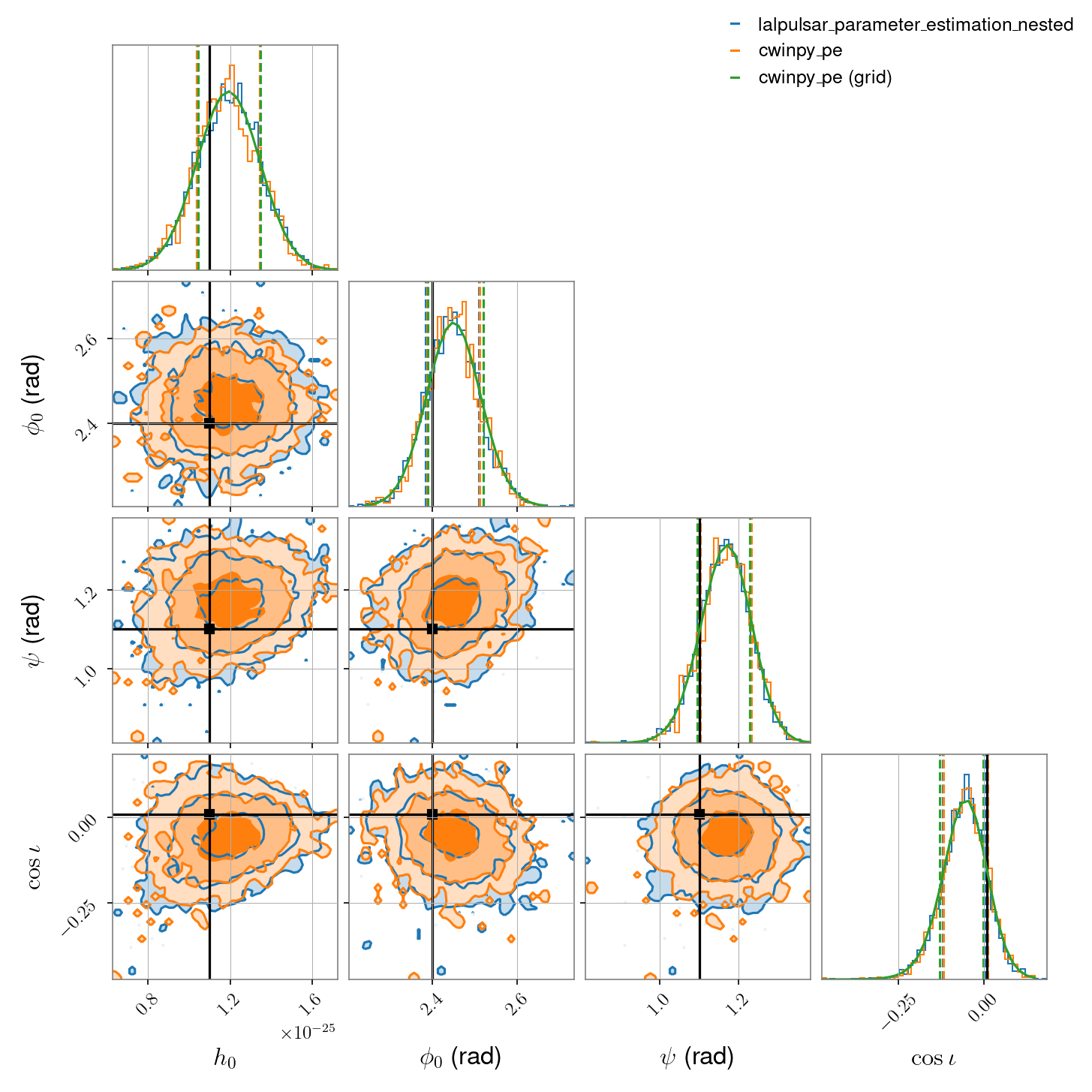
Single detector, software injection (linear polarisation)#

Here we compare lalpulsar_parameter_estimation_nested with cwinpy in the case of simulated Gaussian noise from a single detector (H1 in this case) containing a software injected signal with close-to linear polarisation. The parameters being estimated are \(h_0\), \(\phi_0\), \(\psi\) and \(\cos{\iota}\), all with uniform priors.

The script for this comparison, using the dynesty nested sampling algorithm, is shown at the bottom of the page. It produces the following comparison data:

../_images/single_detector_software_injection_linear_corner.png

Evidence table#
Method	\(\ln{(Z)}\)	\(\ln{(Z)}\) noise	\(\ln{}\) Odds
`lalpulsar_parameter_estimation_nested`	162961.652	162940.311	21.341±0.107
`cwinpy_pe`	162961.875	162940.311	21.564±0.185
`cwinpy_pe` (grid)	162961.593		21.282

Parameter table#
Method	\(h_0\)	\(\phi_0\) (rad)	\(\psi\) (rad)	\(\cos{\iota}\)
`lalpulsar_parameter_estimation_nested`	1.19±0.16×10^-25	2.45±0.06	1.16±0.06	-0.06±0.07
90% credible intervals	[0.94, 1.45]×10^-25	[2.34, 2.56]	[1.06, 1.27]	[-0.17, 0.05]
`cwinpy_pe`	1.18±0.15×10^-25	2.45±0.06	1.17±0.07	-0.06±0.07
90% credible intervals	[0.92, 1.44]×10^-25	[2.35, 2.56]	[1.06, 1.28]	[-0.17, 0.05]

Maximum a-posteriori#
Method	\(h_0\)	\(\phi_0\) (rad)	\(\psi\) (rad)	\(\cos{\iota}\)	\(\ln{(L)}\) max
`lalpulsar_parameter_estimation_nested`	1.25×10^-25	2.44	1.17	-0.05	162975.01
`cwinpy_pe`	1.22×10^-25	2.44	1.17	-0.05	162975.02

Combined K-S test p-value: 0.0115

Maximum Jensen-Shannon divergence: 0.0016

CWInPy version: 1.0.0

bilby version: 2.1.1

#!/usr/bin/env python

"""
Compare cwinpy with lalpulsar_parameter_estimation_nested for
data from a single detector detector containing a software injection
with close-to-linear polarisation.
"""

import os
import subprocess as sp

import h5py
import matplotlib
import numpy as np
from astropy.utils.data import download_file
from bilby.core.prior import Uniform
from comparitors import comparisons
from lalinference import LALInferenceHDF5PosteriorSamplesDatasetName
from lalinference.io import read_samples
from matplotlib import pyplot as plt

from cwinpy import HeterodynedData
from cwinpy.pe import pe
from cwinpy.plot import Plot

matplotlib.use("Agg")

# URL for ephemeris files
DOWNLOAD_URL = "https://git.ligo.org/lscsoft/lalsuite/raw/master/lalpulsar/lib/{}"

# create a fake pulsar parameter file
parcontent = """\
PSRJ     J0123+3456
RAJ      01:23:45.6789
DECJ     34:56:54.321
F0       567.89
F1       -1.2e-12
PEPOCH   56789
H0       1.1e-25
COSIOTA  0.01
PSI      1.1
PHI0     2.4
"""

injection_parameters = {}
injection_parameters["h0"] = 1.1e-25
injection_parameters["phi0"] = 2.4
injection_parameters["psi"] = 1.1
injection_parameters["cosiota"] = 0.01

label = "single_detector_software_injection_linear"
outdir = "outputs"

if not os.path.isdir(outdir):
    os.makedirs(outdir)

# add content to the par file
parfile = os.path.join(outdir, "{}.par".format(label))
with open(parfile, "w") as fp:
    fp.write(parcontent)

# create some fake heterodyned data
detector = "H1"  # the detector to use
asd = 1e-24  # noise amplitude spectral density
times = np.linspace(1000000000.0, 1000086340.0, 1440)  # times
het = HeterodynedData(
    times=times,
    par=parfile,
    injpar=parfile,
    inject=True,
    fakeasd=asd,
    detector=detector,
)

# output the data
hetfile = os.path.join(outdir, "{}_data.txt".format(label))
het.write(hetfile)

# create priors
phi0range = [0.0, np.pi]
psirange = [0.0, np.pi / 2.0]
cosiotarange = [-1.0, 1.0]
h0range = [0.0, 1e-23]

# set prior for lalpulsar_parameter_estimation_nested
priorfile = os.path.join(outdir, "{}_prior.txt".format(label))
priorcontent = """H0 uniform {} {}
PHI0 uniform {} {}
PSI uniform {} {}
COSIOTA uniform {} {}
"""
with open(priorfile, "w") as fp:
    fp.write(priorcontent.format(*(h0range + phi0range + psirange + cosiotarange)))

# set prior for bilby
priors = {}
priors["h0"] = Uniform(h0range[0], h0range[1], "h0", latex_label=r"$h_0$")
priors["phi0"] = Uniform(
    phi0range[0], phi0range[1], "phi0", latex_label=r"$\phi_0$", unit="rad"
)
priors["psi"] = Uniform(
    psirange[0], psirange[1], "psi", latex_label=r"$\psi$", unit="rad"
)
priors["cosiota"] = Uniform(
    cosiotarange[0], cosiotarange[1], "cosiota", latex_label=r"$\cos{\iota}$"
)

# run lalpulsar_parameter_estimation_nested
try:
    execpath = os.environ["CONDA_PREFIX"]
except KeyError:
    raise KeyError(
        "Please work in a conda environment with lalsuite and cwinpy installed"
    )

execpath = os.path.join(execpath, "bin")

lppen = os.path.join(execpath, "lalpulsar_parameter_estimation_nested")
n2p = os.path.join(execpath, "lalinference_nest2pos")

Nlive = 1000  # number of nested sampling live points
Nmcmcinitial = 0  # set to 0 so that prior samples are not resampled

outfile = os.path.join(outdir, "{}_nest.hdf".format(label))

# set ephemeris files
efile = download_file(DOWNLOAD_URL.format("earth00-40-DE405.dat.gz"), cache=True)
sfile = download_file(DOWNLOAD_URL.format("sun00-40-DE405.dat.gz"), cache=True)
tfile = download_file(DOWNLOAD_URL.format("te405_2000-2040.dat.gz"), cache=True)

# set the command line arguments
runcmd = " ".join(
    [
        lppen,
        "--verbose",
        "--input-files",
        hetfile,
        "--detectors",
        detector,
        "--par-file",
        parfile,
        "--prior-file",
        priorfile,
        "--Nlive",
        "{}".format(Nlive),
        "--Nmcmcinitial",
        "{}".format(Nmcmcinitial),
        "--outfile",
        outfile,
        "--ephem-earth",
        efile,
        "--ephem-sun",
        sfile,
        "--ephem-timecorr",
        tfile,
    ]
)

with sp.Popen(
    runcmd,
    stdout=sp.PIPE,
    stderr=sp.PIPE,
    shell=True,
    bufsize=1,
    universal_newlines=True,
) as p:
    for line in p.stderr:
        print(line, end="")

# convert nested samples to posterior samples
outpost = os.path.join(outdir, "{}_post.hdf".format(label))
runcmd = " ".join([n2p, "-p", outpost, outfile])
with sp.Popen(
    runcmd,
    stdout=sp.PIPE,
    stderr=sp.PIPE,
    shell=True,
    bufsize=1,
    universal_newlines=True,
) as p:
    for line in p.stdout:
        print(line, end="")

# get posterior samples
post = read_samples(outpost, tablename=LALInferenceHDF5PosteriorSamplesDatasetName)
lp = len(post["H0"])
postsamples = np.zeros((lp, len(priors)))
for i, p in enumerate(priors.keys()):
    postsamples[:, i] = post[p.upper()]

# get evidence
hdf = h5py.File(outpost, "r")
a = hdf["lalinference"]["lalinference_nest"]
evsig = a.attrs["log_evidence"]
evnoise = a.attrs["log_noise_evidence"]
hdf.close()

# run bilby via the pe interface
runner = pe(
    data_file=hetfile,
    par_file=parfile,
    prior=priors,
    detector=detector,
    outdir=outdir,
    label=label,
)

result = runner.result

# evaluate the likelihood on a grid
gridpoints = 30
grid_size = dict()
for p in priors.keys():
    grid_size[p] = np.linspace(
        np.min(result.posterior[p]), np.max(result.posterior[p]), gridpoints
    )

grunner = pe(
    data_file=hetfile,
    par_file=parfile,
    prior=priors,
    detector=detector,
    outdir=outdir,
    label=label,
    grid=True,
    grid_kwargs={"grid_size": grid_size},
)

grid = grunner.grid

# output comparisons
comparisons(label, outdir, grid, priors, cred=0.9)

# create results plot
allresults = {
    "lalpulsar_parameter_estimation_nested": outpost,
    "cwinpy_pe": result,
    "cwinpy_pe (grid)": grid,
}

colors = {
    key: plt.rcParams["axes.prop_cycle"].by_key()["color"][i]
    for i, key in enumerate(allresults.keys())
}

plot = Plot(
    results=allresults,
    parameters=list(priors.keys()),
    plottype="corner",
    pulsar=parfile,
)

plot.plot(
    bins=50,
    smooth=0.9,
    quantiles=[0.16, 0.84],
    levels=(1 - np.exp(-0.5), 1 - np.exp(-2), 1 - np.exp(-9 / 2.0)),
    fill_contours=True,
    colors=colors,
)

plot.savefig(os.path.join(outdir, "{}_corner.png".format(label)), dpi=150)