Known pulsar parameter estimation

CWInPy can be used for perform Bayesian inference on gravitational-wave data to estimate the gravitational-wave signal parameters for emission from a known pulsar. To sample from the joint parameter posterior distributions, CWInPy uses the bilby package as an interface to a variety of stochastic sampling methods.

CWInPy comes with an executable, cwinpy_pe, for performing this analysis, which tries to emulate, as much as possible, the functionality from the LALSuite code lalpulsar_parameter_estimation_nested (formerly lalapps_pulsar_parameter_estimation_nested) described in [1].

There is also an API for running this analysis from within a Python shell or script as described below.

Running the analysis

The cwinpy_pe executable, and API, can be used to perform parameter estimation over a variety of signal parameter both on real data or simulated data. We will cover some examples of both cases and show equivalent ways of running the analysis via the use of: command line arguments to the cwinpy_pe executable, a configuration file, or the API. The current command line arguments for cwinpy_pe are given below.

Example: single detector data

In the first example we will show how to perform parameter estimation on some real gravitational-wave data. We will use a short segment of data from the O1 run of the LIGO detectors (the whole of which can be found on the GWOSC website) between GPS times of 1132444817 and 1136419217. The O1 dataset contains a set of simulated pulsar signals that have been “injected” into it. We will look at the injected signal named PULSAR8, the parameters of which can be found at this link.

The data we will use in this example is from the LIGO Hanford detector (abbreviated to “H1”) and has been heterodyned using the known phase evolution of the simulated signal (see the description here), and low-pass filtered and down-sampled to a rate of one sample per minute. This data file (in a gzipped format) can be downloaded here: fine-H1-PULSAR08.txt.gz.

A Tempo(2)-style [2] pulsar parameter (.par) file for this simulated signal is reproduced below and can be downloaded here, where it should be noted that the F0 and F1 parameters in that file are the expected rotation frequency and frequency derivative of the putative pulsar, so they are half those of the simulated gravitational-wave signal in the data.

NAME JPULSAR08
PSRJ JPULSAR08
F0	97.15415925
F1	-4.325e-09
RAJ	23:25:33.4997197871
DECJ	-33:25:06.6608320859
PEPOCH	52944.0007428703684126958
UNITS TDB
H0 1.10013760155e-24
PSI 0.170470927
PHI0 2.945
COSIOTA 0.073902656035643471

Here we will try and estimate four of the signal’s parameters: the gravitational-wave amplitude \(h_0\); the inclination angle \(\iota\) of the rotation axis to the line-of-sight; the initial rotational phase of the signal \(\phi_0\); and the polarisation angle of the source \(\psi\). To do this we have to define a file containing the prior probability distributions for these parameters. We can define the priors in a file as described in the documentation for the bilby package, which is reproduced below and can be downloaded here:

# define priors on: the gravitational-wave amplitude, inclination angle,
# initial phase and polarisation angle
h0 = Uniform(name='h0', minimum=0, maximum=1e-22, latex_label='$h_0$')
iota = Sine(name='iota', minimum=0., maximum=np.pi, latex_label='$\iota$', unit='rad')
phi0 = Uniform(name='phi0', minimum=0, maximum=np.pi, latex_label='$\phi_0$', unit='rad')
psi = Uniform(name='psi', minimum=0, maximum=np.pi / 2, latex_label='$\psi$', unit='rad')

Here we have set the prior on \(h_0\) to be uniform between 0 and 10^-22, where in this case the maximum has been chosen to be large compared to the expected signal strength. The combination of the \(\iota\) and \(\psi\) parameters has been chosen to be uniform over a sphere, which means using a uniform prior over \(\psi\) between 0 and \(\pi/2\) (there is a degeneracy meaning this doesn’t have to cover the full range between 0 and \(2\pi\) [1] [3]), and a sine distribution prior on \(\iota\) (equivalently one could use a uniform prior on a \(\cos{\iota}\) parameter between -1 and 1). The \(\phi_0\) parameter is the initial rotational phase at a given epoch, so only needs to span 0 to \(\pi\) to cover the full phase of the equivalent gravitational-wave phase parameter in the case where the source is emitting at twice the rotational frequency.

With the data at hand, and the priors defined, the analysis can now be run. It is recommended to run by setting up a configuration file, although as mentioned equivalent command line arguments can be passed to cwinpy_pe (or a combination of a configuration file and command line arguments may be useful if defining some fixed setting for many analyses in the file, but making minor changes for individual cases on the command line). A configuration file for this example is shown below, with comments describing the parameters given inline:

# configuration file for Example 1

# The path to the TEMPO(2)-style pulsar parameter file
par-file=PULSAR08.par

# The name of the detector from which the data comes
detector=H1

# The path to the data file for the given detector. This could equivalently be
# given (and the 'detector' argument omitted) with:
# data-file=[H1:fine-H1-PULSAR08.txt.gz]
# or
# data-file={'H1': 'fine-H1-PULSAR08.txt.gz'}
# or using the 'data-file-2f' argument to be explicit about the
# gravitational-wave frequency being two times the rotation frequency
data-file=fine-H1-PULSAR08.txt.gz

# The output directory for the results (this will be created if it does not exist)
outdir=example1

# A prefix for the results file name
label=example1

# The Bayesian stochastic sampling algorithm (defaults to dynesty if not given)
sampler=dynesty

# Keyword arguments for the sampling algorithm
sampler-kwargs={'Nlive': 1000, 'plot': True}

# Show "true" signal values on the output plot (as we know this data contains a simulated signal!)
show-truths = True

# The path to the prior file
prior=example1_prior.txt

Note

When using the dynesty sampler (as wrapped through bilby) it will default to use the rwalk sampling method. This has been found to work well and be the quickest option for normal running. A discussion of the bilby-specific different dynesty sampling options can be found here, while discussion of the options in dynesty itself can be found here.

The analysis can then be run using:

cwinpy_pe --config example1_config.ini

which should only take a few minutes, with information on the run output to the terminal.

This will create a directory called example1 containing: the results as a bilby Results object saved, by default, in an HDF5 format file called example1_result.hdf5 (see here for information on reading this information within Python); and (due to the setting of 'plot': True in the sampler_kwargs dictionary), a “corner plot” in the file example1_corner.png showing 1D and 2D marginalised posterior probability distributions for each parameter, and pair of parameters. To instead save the results to a JSON format file you would include "save": "json" in the sampler_kwargs dictionary. To gzip the JSON file you would include "gzip": True in the sampler_kwargs dictionary.

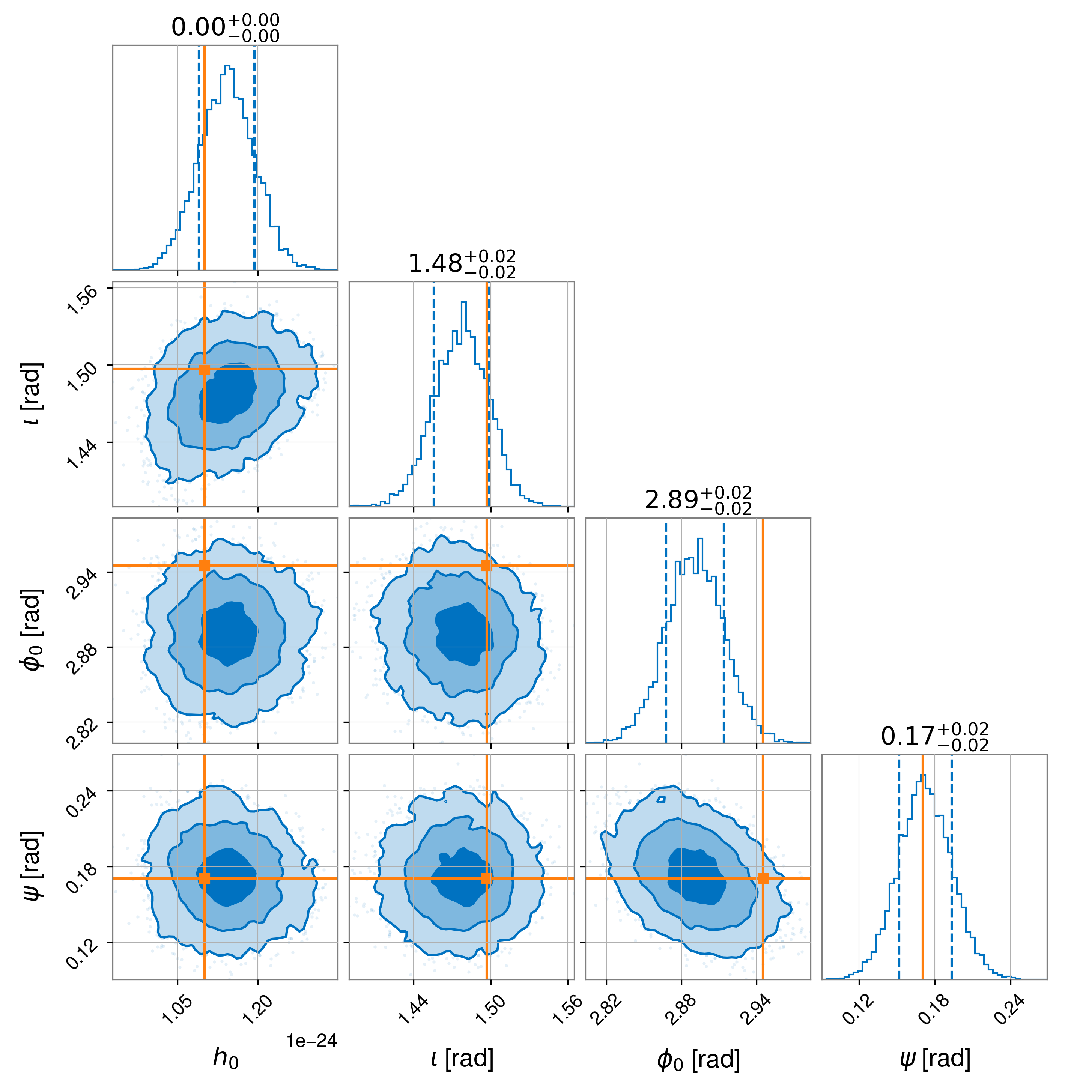
Note

The slight offset seen in the recovered phase is related to the uncompensated 150 microsec time delay in the actuation function used to generate the simulated signal as discussed in [4].

The code should also output the natural logarithm of the signal model evidence (log_evidence), noise-only model evidence (log_noise_evidence), and Bayes factor between those two models, and estimates of the uncertainties on the signal model evidence.

log_noise_evidence: 869768.909
log_evidence: 870014.455 ± 0.180
log_bayes_factor: 245.547 ± 0.180

If running the example you should find an identical noise evidence value, although the signal model evidence, and therefore Bayes factor, and its uncertainty may vary slightly due to the stochastic nature of the sampling process. These values can also be extracted from the results file called example1_result.hdf5.

Rather than using the configuration file, all the arguments could be given on the command line (although using the configuration file is highly recommended), with the following command:

cwinpy_pe --detector H1 --par-file PULSAR08.par --data-file fine-H1-PULSAR08.txt.gz --outdir example1 --label example1 --sampler dynesty --sampler-kwargs "{'Nlive':1000,'sample':'rwalk','plot':True}" --prior example1_prior.txt --show-truths

where it should be noted that the --sampler-kwargs dictionary argument must be given within quotation marks.

Example: multi-detector data

In this example we will replicate the analysis from the first example, but will use O1 data from more than one detector. It will again look at the hardware injection signal named PULSAR8 and use the same parameter file as given above.

The data we will use in this example is a short segment (between GPS times of 1132444817 and 1136398891) from both the LIGO Hanford detector (abbreviated to “H1”) and the LIGO Livingston detector (abbreviated to “L1”). Both sets of data have been heterodyned using the known phase evolution of the simulated signal (see the description here), and low-pass filtered and down-sampled to a rate of one sample per minute. The data files (in a gzipped format) can be downloaded here: fine-H1-PULSAR08.txt.gz and fine-L1-PULSAR08.txt.gz. We will use an identical prior file to that in the first example, but rename it example2_prior.txt.

The configuration file for this example is shown below, with comments describing the parameter given inline:

# configuration file for Example 2

# The path to the TEMPO(2)-style pulsar parameter file
par-file=PULSAR08.par

# The name of the detectors from which the data comes
detector=[H1, L1]

# The path to the data file for the given detector. This could equivalently be
# given (and the 'detector' argument omitted) with:
# data-file=[H1:fine-H1-PULSAR08.txt.gz, L1:fine-L1-PULSAR08.txt.gz]
# or
# data-file={'H1': 'fine-H1-PULSAR08.txt.gz', 'L1': 'fine-L1-PULSAR08.txt.gz'}
# or using the 'data-file-2f' argument to be explicit about the
# gravitational-wave frequency being two times the rotation frequency
data-file=[fine-H1-PULSAR08.txt.gz, fine-L1-PULSAR08.txt.gz]

# The output directory for the results (this will be created if it does not exist)
outdir=example2

# A prefix for the results file name
label=example2

# The Bayesian stochastic sampling algorithm (defaults to dynesty if not given)
sampler=dynesty

# Keyword arguments for the sampling algorithm
sampler-kwargs={'Nlive': 1000, 'plot': True}

# Show "true" signal values on the output plot (as we know this data contains a simulated signal!)
show-truths = True

# The path to the prior file
prior=example2_prior.txt

The analysis can then be run using:

cwinpy_pe --config example2_config.ini

This will create a directory called example2 containing: the results as a bilby Results object saved, by default, in an HDF5 format file called example2_result.hdf5 (see here for information on reading this information within Python); and (due to the setting of 'plot': True in the sampler_kwargs dictionary), a “corner plot” in the file example2_corner.png showing 1D and 2D marginalised posterior probability distributions for each parameter, and pair of parameters.

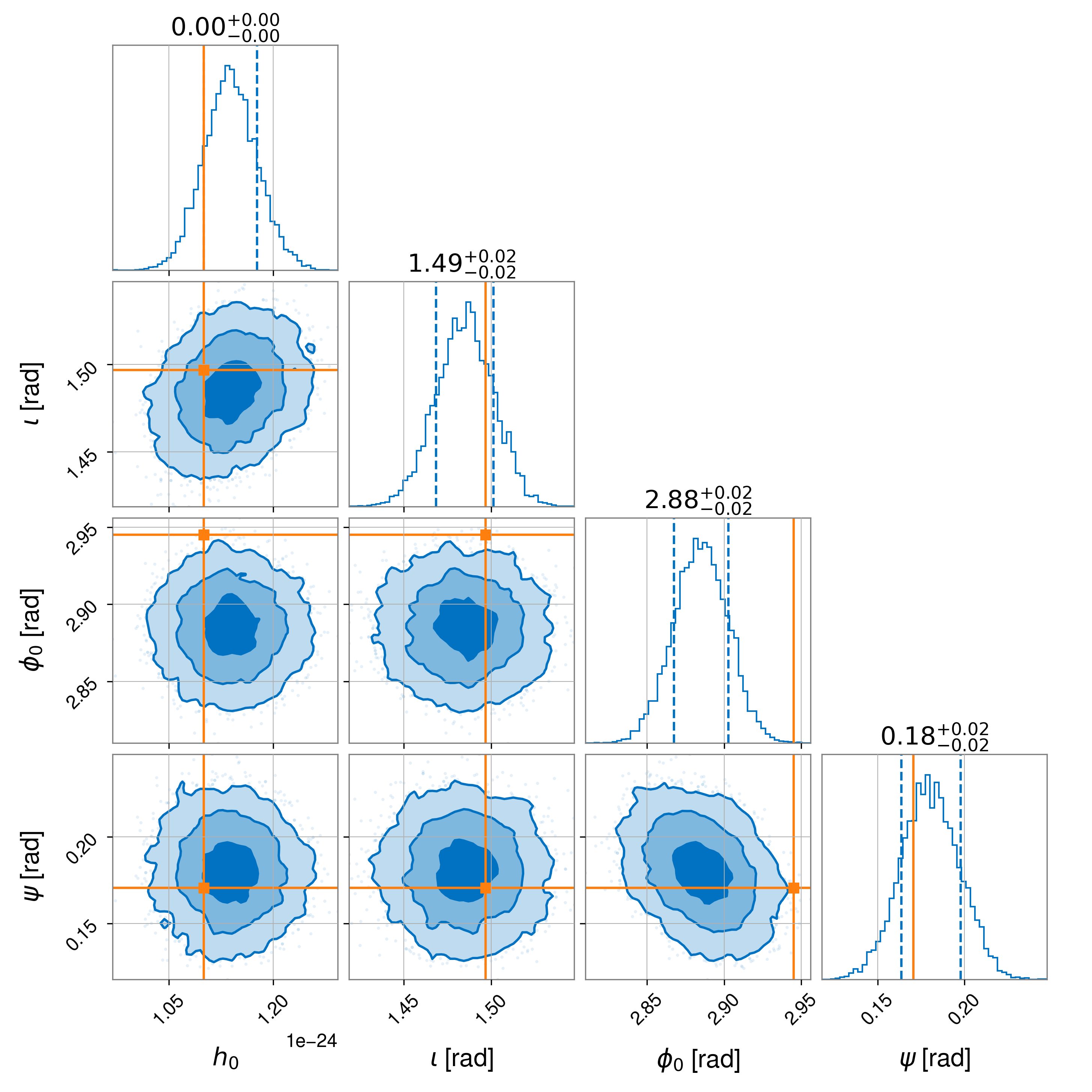
Note

The slight offset seen in the recovered phase is related to the uncompensated 150 microsec time delay in the actuation function used to generate the simulated signal as discuss in [4].

The natural logarithms of the signal model evidence (log_evidence), noise-only model evidence (log_noise_evidence) and Bayes factor (log_bayes_factor) output for this example are

log_noise_evidence: 1492439.107
log_evidence: 1492888.344 ± 0.186
log_bayes_factor: 449.237 ± 0.186

If running the example you should find an identical noise evidence value, although the signal model evidence, and therefore Bayes factor, and its uncertainty may vary slightly due to the stochastic nature of the sampling process. These values can also be extracted from the results file called example2_result.hdf5.

The equivalent full command line arguments that could be used are:

cwinpy_pe --detector H1 --detector L1 --par-file PULSAR08.par --data-file fine-H1-PULSAR08.txt.gz --data-file fine-L1-PULSAR08.txt.gz --outdir example2 --label example2 --sampler dynesty --sampler-kwargs "{'Nlive':1000,'sample':'rwalk','plot':True}" --prior example2_prior.txt --show-truths

Example: a simulated transient-continuous signal

It is interesting to consider signals that do not have a constant amplitude, but are transitory on time scales of days-to-weeks-months (e.g., [8], [9], [10]); so-called “transient-continuous” signals. These might occur following a pulsar glitch [11]. CWInPy is able to simulate and infer the parameters of two classes of these signals, which use the normal continuous signal model modulated by a particular window function:

1. a rectangular window where the signal abruptly turns on then off;

2. an exponentially decaying window, where there is an abrupt start followed by an exponential decay.

Both models are defined by a start time, e.g., the time of an observed pulsar glitch, and a timescale \(\tau\), which defines the duration of the rectangular window model and the decay time constant for the exponential window model.

In this example, we will simulate a transient signal with a rectangular window in data from the both the LIGO Hanford detector (abbreviated to “H1”) and the LIGO Livingston detector between 01:46:25 on 14th Sept 2011 (a GPS time of 1000000000) and 01:46:25 on 18th Sept 2011.

To simulate a transient signal, the Tempo(2)-style pulsar parameter (.par) file needs to contain the following parameters:

• TRANSIENTWINDOWTYPE: this can be RECT (rectangular window) or EXP (exponential window);

• TRANSIENTSTARTTIME: the time at which the signal “turns-on”. This should be give as in Modified Julian Day (MJD) format, which is how glitch times are defined in Tempo(2);

• TRANSIENTTAU: the signal duration (rectangular window) or decay time constant (exponential window) in days.

For this example, the .par file we used defined a model with a rectangular window. It and can be downloaded here and is reproduced below.

NAME JTRANSIENT
PSRJ JTRANSIENT
F0	234.5678
F1	-1.34e-11
RAJ	03:25:33.5
DECJ	-13:25:07.9
PEPOCH	56786
H0       1.8e-25
COSIOTA  -0.45
PSI      1.1
PHI0     2.4
TRANSIENTWINDOWTYPE RECT
TRANSIENTSTARTTIME  55818.573900462965
TRANSIENTTAU        1.5

To estimate the parameters of the transient signal model they must be included in the file defining the required prior probability distributions. The prior file we use is reproduced below and can be downloaded here:

# define priors on: the gravitational-wave amplitude, inclination angle,
# initial phase and polarisation angle
h0 = Uniform(name='h0', minimum=0, maximum=1e-22, latex_label='$h_0$')
iota = Sine(name='iota', minimum=0., maximum=np.pi, latex_label='$\iota$', unit='rad')
phi0 = Uniform(name='phi0', minimum=0, maximum=np.pi, latex_label='$\phi_0$', unit='rad')
psi = Uniform(name='psi', minimum=0, maximum=np.pi / 2, latex_label='$\psi$', unit='rad')
transientstarttime = Gaussian(name='transientstarttime', mu=55818.573900462965, sigma=0.5, latex_label='$t_0$', unit='d')
transienttau = Uniform(name='transienttau', minimum=0.1, maximum=3.0, latex_label='$\\tau$', unit='d')

If setting the TRANSIENTSTARTTIME and TRANSIENTTAU to use MJD and days, respectively, in the prior file (to be consistent with the .par file) then the unit key for each prior must be set to d (for day). Otherwise the values will be expected in GPS seconds and seconds. In this case, a Gaussian prior is used for the start time with a mean given by the actual simulated start time and a standard deviation of 0.5 days, and a uniform prior is used for the duration within a range from 0.1 to 3 days.

Note

You can use the astropy.time.Time class to convert between GPS and MJD, e.g.:

>>> from astropy.time import Time
>>> mjd = Time(1234567890, format="gps", scale="tdb").mjd

or vice versa:

>>> gps = Time(1234567890, format="mjd", scale="tdb").gps

A configuration file that can be passed to cwinpy_pe for this example is shown below, with comments describing the parameters given inline:

# configuration file for Example 3

# The paths to the TEMPO(2)-style injection file
par-file=TRANSIENT.par
inj-par=TRANSIENT.par

# The start and end times of the simulated data
fake-start=1000000000
fake-end=1000345600

# Use design curve ASD for simulated noise
fake-asd=[H1, L1]

# The output directory for the results (this will be created if it does not exist)
outdir=example3

# A prefix for the results file name
label=example3

# The Bayesian stochastic sampling algorithm (defaults to dynesty if not given)
sampler=dynesty

# Keyword arguments for the sampling algorithm
sampler-kwargs={'Nlive': 1000, 'plot': True}

# Show "true" signal values on the output plot (as we know this data contains a simulated signal!)
show-truths = True

# The path to the prior file
prior=example3_prior.txt

This can then be run with:

cwinpy_pe --config example3_config.ini

which produces the following posteriors:

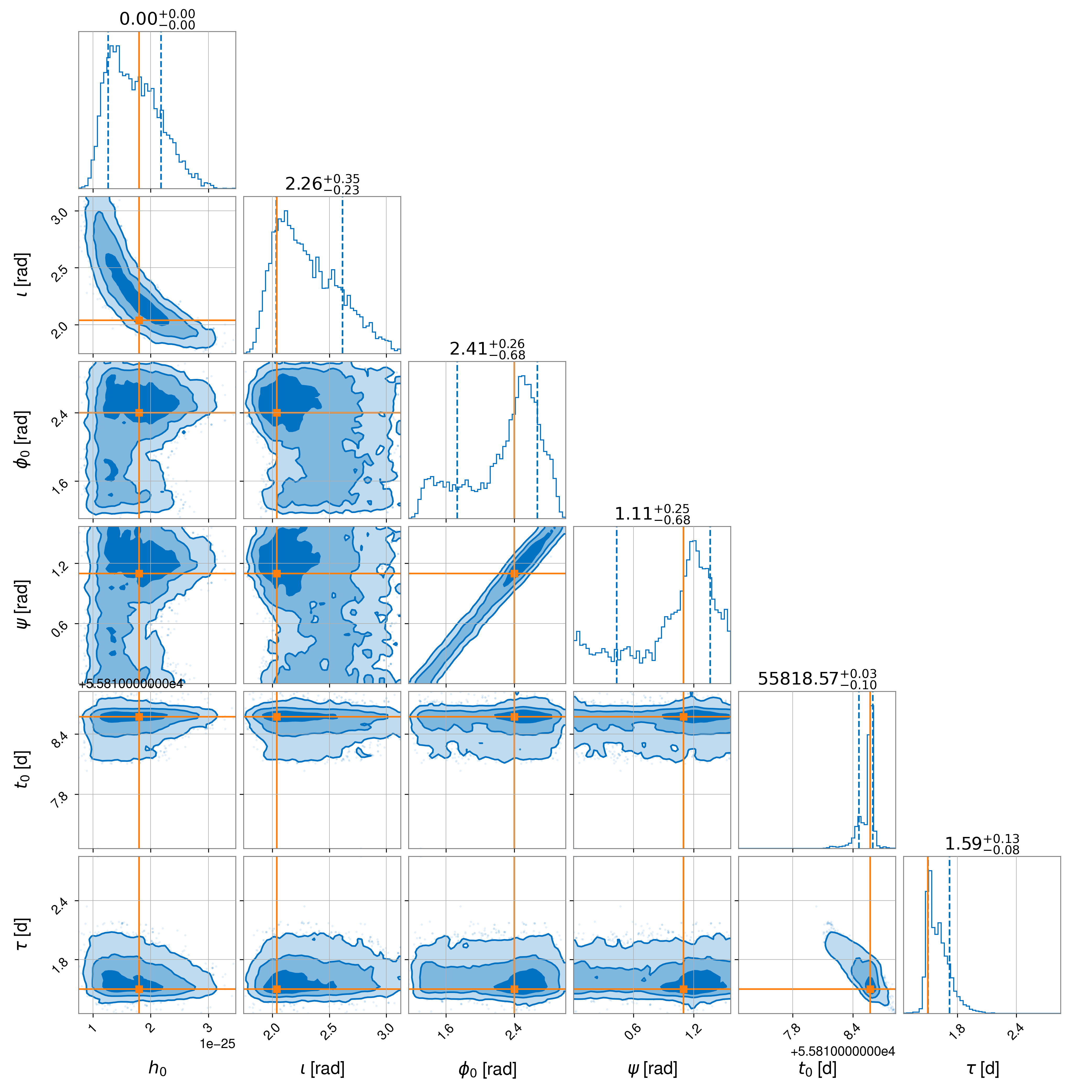
and the following signal model and noise model log evidence values:

ln_noise_evidence: 1274081.150
ln_evidence: 1274102.482 +/-  0.189
ln_bayes_factor: 21.331 +/-  0.189

Running on multiple sources

You may have multiple real sources for which you want to perform parameter estimation, or you may want to simulate data from many sources. If you have a multicore machine or access to a computer cluster with HTCondor installed you can use CWInPy to create a set of analysis jobs, in the form of an HTCondor DAG, for each source. This makes use of PyCondor, which is installed as one of the requirements for CWInPy.

To set up a DAG to analyse real data for multiple pulsars you need to have certain datasets and files organised in a particular way. You must have a set of Tempo(2)-style pulsar parameter files, with only one for each pulsar you wish to analyse, which each contain a PSRJ value giving the pulsar’s name, e.g.,

PSRJ  J0534+2200

You also need to have a directory structure where the heterodyned data (see here) from individual detectors are in distinct directories (if you want specify each file for each pulsar individually in a dictionary this can be done instead, but requires more manual editing). Also, if there is data from both the a potential signal at the sources rotation frequency and twice the rotation frequency, then these should also be in distinct directories. The heterodyned data file for a particular pulsar must contain the PSRJ name of the pulsar, as given in the associated parameter file, either in the file name or the file directory path.

An example of such a directory tree structure might be:

root
 ├── pulsars              # directory containing pulsar parameter files
 ├── priors               # directory containing pulsar prior distribution files
 ├── detector1            # directory containing data for first detector
 |    ├── 1f              # directory containing data from first detector at the source rotation frequency
 |    |    ├── pulsar1    # directory containing data from first detector, at the rotation frequency for first pulsar (could be named using the pulsar's PSRJ name)
 |    |    ├── pulsar2    # directory containing data from first detector, at the rotation frequency for second pulsar (could be named using the pulsar's PSRJ name)
 |    |    └── ...
 |    └── 2f
 |         ├── pulsar1    # directory containing data from first detector, at twice the rotation frequency for first pulsar (could be named using the pulsar's PSRJ name)
 |         ├── pulsar2    # directory containing data from first detector, at twice the rotation frequency for second pulsar (could be named using the pulsar's PSRJ name)
 |         └── ...
 ├── detector2            # directory contain data for second detector
 |    └── ...
 └── ...

The DAG for the analysis can be created using the cwinpy_pe_pipeline executable, which requires a configuration file as its only input. An example configuration file, based on the above directory tree structure is given below. Comments about each input parameter, and different potential input options are given inline; some input parameters are also commented out using a ; if the default values are appropriate. For more information on the various HTCondor options see the user manual.

[run]
# the base directory for the analysis **output**
basedir = root

######### Condor DAG specific inputs ########
[pe_dag]
# the location of the directory to contain the Condor DAG submission files
# (defaults to "basedir/submit")
;submit = 

# the prefix of the name for the Condor DAGMan submit file (defaults to
# "dag_cwinpy_pe"). "dag" will always be prepended.
;name =

# a flag specifying whether to automatically submit the DAG after its creation
# (defaults to False)
submitdag = False

# a flag saying whether to build the DAG (defaults to True)
;build =

# set whether running on the OSG (defaults to False). If using the OSG it
# expects you to be within an IGWN conda environment or using the singularity
# container option below.
;osg =

# if wanting to run on the OSG with the latest development version of cwinpy,
# which is within a Singularity container, set this flag to True
;singularity

# if running on the OSG you can select desired sites to run on
# see https://computing.docs.ligo.org/guide/condor/submission/#DESIRED_Sites
;desired_sites =
;undesired_sites =

######## cwinpy_pe Job options ########
[pe_job]
# the location of the cwinpy_pe executable to use (defaults to try and find
# cwinpy_pe in the current user PATH)
;executable =

# set the Condor universe (defaults to "vanilla") 
;universe =

# directory location for the output from stdout from the Job (defaults to
# "basedir/log")
;out =

# directory location for the output from stderr from the Job (defaults to
# "basedir/log")
;error =

# directory location for any logging information from the jobs (defaults to
# "basedir/log")
;log =

# the location of the directory to contain the Condor job submission files
# (defaults to "basedir/submit")
;submit =

# the amount of available memory request for each job (defaults to 4 Gb)
# [Note: this is required for vanilla jobs on LIGO Scientific Collaboration
# computer clusters]
;request_memory =

# the amount of disk space required for each job (defaults to 1 Gb)
# [Note: this is required for vanilla jobs on LIGO Scientific Collaboration
# computer clusters]
;request_disk =

# the number of CPUs the job requires (defaults to 1, cwinpy_pe is not
# currently parallelised in any way)
;request_cpus =

# additional Condor job requirements (defaults to None)
;requirements =

# set how many times the DAG will retry a job on failure (default to 2)
;retry =

# Job accounting group and user [Note: these are required on LIGO Scientific
# Collaboration computer cluster, but may otherwise be left out, see
; https://accounting.ligo.org/user for valid accounting tags]
;accounting_group =
accounting_group_user = albert.einstein

####### Source and solar system ephemeride files ##########
[ephemerides]
# The pulsar parameter files, where all files are expected to have the
# extension ".par". This can either be:
#  - the path to a single file (if running with a single source)
#  - a list of parameter files
#  - a directory (or glob-able directory pattern) containing parameter files
#  - a combination of a list of directories and/or files
pulsars = /root/pulsars

# Pulsar "injection" parameter files containing simulated signal parameters to
# add to the data. If not given then no injections will be performed. If given
# it should be in the same style as the "pulsars" section.
;injections =

# Locations of the Earth and Sun ephemerides. If not given then the ephemerides
# will be automatically determined from the pulsar parameter information. The
# values should be dictionaries keyed to the ephemeris type, e.g., "DE405", and
# pointing to the location of the ephemeris file.
;earth =
;sun =

######## PE specific options ########
[pe]

# The number of parallel runs for each pulsar. These will be combined to
# create the final output. This defaults to 1.
;n_parallel =

# The period for automatically restarting HTCondor PE jobs to prevent a hard
# eviction. If not given this defaults to 43200 seconds
;periodic-restart-time =

# The directory within basedir into which to output the results in individual
# directories named using the PSRJ name (defaults to "results")
;results =

# Locations of heterodyned data files produced at twice the rotation frequency
# of the source. This must be a dictionary keyed to detector names. The value
# of each detector-keyed item can be:
#  - the path to a single file (if analysing one detector)
#  - a directory (or glob-able directory pattern) containing (only) data files
#  - a list of files (or directories/directory patterns)
#  - a dictionary keyed to pulsar PSRJ names containing the full paths to the
#    associated data file
# The file name or path for each dataset must contain the associated pulsar
# PSRJ name.
# This can alternatively be just given as "data-file"
data-file-2f = {"H1": "/root/detector1/2f/*/*", "L1": "/root/detector2/2f/*/*"}

# Locations of heterodyned data files produced at the rotation frequency of the
# source (if required). This must be a dictionary keyed to detector names. The value of each
# detector-keyed item can be:
#  - the path to a single file (if analysing one detector)
#  - a directory (or glob-able directory pattern) containing (only) data files
#  - a list of files (or directories/directory patterns)
#  - a dictionary keyed to pulsar PSRJ names containing the full paths to the
#    associated data file
# The file name or path for each dataset must contain the associated pulsar
# PSRJ name. [Note: this is not required if only analysing data at twice the
# rotation frequency]
data-file-1f = {"H1": "/root/detector1/1f/*/*", "L1": "/root/detector2/1f/*/*"}

# Set a dictionary of keyword arguments to be used by the HeterodynedData class
# that the data files will be read into.
;data_kwargs = {}

# Set this boolean flag to state whether to run parameter estimation with a
# likelihood that uses the coherent combination of data from all detectors
# specified. This defaults to True.
;coherent =

# Set this boolean flag to state whether to run the parameter estimation for
# each detector independently. This defaults to False.
;incoherent =

# Flags to set to generate simulated Gaussian noise to analyse, if data files
# are not given. "fake-asd-1f" is used to produce simulated noise at the source
# rotation frequency and "fake-asd-2f" (or just "fake-asd" is used to produce
# simulated noise at twice the source rotation frequency). The values these can
# take are:
#  - a list of detectors, in which case the detector's design sensitivity curve
#    will be used when generating the noise for each pulsar
#  - a dictionary, keyed to detector names, either giving a value that is an
#    amplitude spectral density value to be used, or a file containing a
#    frequency series of amplitude spectral densities to use
;fake-asd-1f =
;fake-asd-2f =

# Flags to set the start time, end time time step and random seed for the fake
# data generation. Either both 'fake-start' and 'fake-end' must be set, or
# neither should be set. Each of the time values can either be:
#  - a single integer or float giving the GPS time/time step
#  - a dictionary keyed to the detector names containing the value for the
#    given detector
# If not given the fake data for any required detectors will start at a GPS
# time of 1000000000 and end at 1000086400 (i.e., for one day), with a time
# step of 60 seconds
;fake-start =
;fake-end =
;fake-dt =
;fake-seed =

# The prior distributions to use for each pulsar. The value of this can either
# be:
#  - a single prior file (in bilby format) to use for all pulsars
#  - a list of prior files, where each filename contains the PSRJ name of the
#    associated pulsar
#  - a directory, or glob-able directory pattern, containing the prior files,
#    where each filename contains the PSRJ name of the associated pulsar
#  - a dictionary with prior file names keyed to the associated pulsar
# If not given then default priors will be used. If using data at just twice
# the rotation frequency the default priors are:
#   h0 = Uniform(minimum=0.0, maximum=1.0e-22, name='h0')
#   phi0 = Uniform(minimum=0.0, maximum=pi, name='phi0')
#   iota = Sine(minimum=0.0, maximum=pi, name='iota')
#   psi = Uniform(minimum=0.0, maximum=pi/2, name='psi')
# For data at just the rotation frequency the default priors are:
#   c21 = Uniform(minimum=0.0, maximum=1.0e-22, name='c21')
#   phi21 = Uniform(minimum=0.0, maximum=2*pi, name='phi21')
#   iota = Sine(minimum=0.0, maximum=pi, name='iota')
#   psi = Uniform(minimum=0.0, maximum=pi/2, name='psi')
# And, for data at both frequencies, the default priors are:
#   c21 = Uniform(minimum=0.0, maximum=1.0e-22, name='c21')
#   c22 = Uniform(minimum=0.0, maximum=1.0e-22, name='c22')
#   phi21 = Uniform(minimum=0.0, maximum=2*pi, name='phi21')
#   phi22 = Uniform(minimum=0.0, maximum=2*pi, name='phi22')
#   iota = Sine(minimum=0.0, maximum=pi, name='iota')
#   psi = Uniform(minimum=0.0, maximum=pi/2, name='psi')
priors = /root/priors

# Flag to say whether to output the injected/recovered signal-to-noise ratios
# (defaults to False)
;output_snr =

# The location within basedir for the cwinpy_pe configuration files
# generated to each source (defaults to "configs")
;config =

# The stochastic sampling package to use (defaults to "dynesty")
;sampler =

# A dictionary of any keyword arguments required by the sampler package
# (defaults to None)
;sampler_kwargs =

# A flag to set whether to use the numba-enable likelihood function (defaults
# to True)
;numba =

# A flag to set whether to generate and use a reduced order quadrature for the
# likelihood calculation (defaults to False)
;roq =

# A dictionary of any keyword arguments required by the ROQ generation
;roq_kwargs =

Once the configuration file is created (called, say, cwinpy_pe_pipeline.ini), the Condor DAG dag can be generated with:

cwinpy_pe_pipeline cwinpy_pe_pipeline.ini

This will, using the defaults and values in the above file, generate the following directory tree structure:

root
 ├── results            # directory to contain the results for all pulsars
 |    ├── pulsar1       # directory to contain the results for pulsar1 (named using the PSRJ name)
 |    ├── pulsar1       # directory to contain the results for pulsar2 (named using the PSRJ name)
 |    └── ...
 ├── configs            # directory containing the cwinpy_pe configuration files for each pulsar
 |    ├── pulsar1.ini   # cwinpy_pe configuration file for pulsar1 (named using the PSRJ name)
 |    ├── pulsar2.ini   # cwinpy_pe configuration file for pulsar2 (named using the PSRJ name)
 |    └── ...
 ├── submit             # directory containing the DAG and job submit files
 |    ├── dag_cwinpy_pe.submit      # Condor DAG submit file
 |    ├── cwinpy_pe_H1L1_pulsar1.submit  # cwinpy_pe job submit file for pulsar1
 |    ├── cwinpy_pe_H1L1_pulsar2.submit  # cwinpy_pe job submit file for pulsar2
 |    └── ...
 └── log                # directory for the job log files

By default, if passed data for multiple detectors, the parameter estimation will be performed with a likelihood that coherently combines the data from all detectors. To also include parameter estimation using data from each detector individually, the [pe] section of the configuration file should contain

incoherent = True

The submit files and the final output parameter estimation files will show the combination of detectors used in the filename.

If the original cwinpy_pe_pipeline configuration file contained the line:

submitdag = True

in the [dag] section, then the DAG will automatically have been submitted, otherwise it could be submitted with:

condor_submit_dag /root/submit/dag_cwinpy_pe.submit

Note

If running on LIGO Scientific Collaboration computing clusters the acounting_group value must be specified and be a valid tag. Valid tag names can be found here unless custom values for a specific cluster are allowed.

Command line arguments

The command line arguments for cwinpy_pe can be found using:

$ cwinpy_pe --help
usage: /home/docs/checkouts/readthedocs.org/user_builds/cwinpy/conda/latest/bin/cwinpy_pe
       [-h] [--config CONFIG] [--version]
       [--periodic-restart-time PERIODIC_RESTART_TIME] [--par-file PAR_FILE]
       [-d DETECTOR] [--data-file DATA_FILE] [--data-file-2f DATA_FILE_2F]
       [--data-file-1f DATA_FILE_1F] [--data-kwargs DATA_KWARGS]
       [--inj-par INJ_PAR] [--inj-times INJ_TIMES] [--show-truths]
       [--fake-asd FAKE_ASD] [--fake-asd-1f FAKE_ASD_1F]
       [--fake-asd-2f FAKE_ASD_2F] [--fake-sigma FAKE_SIGMA]
       [--fake-sigma-1f FAKE_SIGMA_1F] [--fake-sigma-2f FAKE_SIGMA_2F]
       [--fake-start FAKE_START] [--fake-end FAKE_END] [--fake-dt FAKE_DT]
       [--fake-seed FAKE_SEED] [-o OUTDIR] [-l LABEL] [--output-snr]
       [-s SAMPLER] [--sampler-kwargs SAMPLER_KWARGS]
       [--likelihood LIKELIHOOD] [--disable-numba] [--usetempo2] --prior PRIOR
       [--grid] [--grid-kwargs GRID_KWARGS] [--roq] [--roq-kwargs ROQ_KWARGS]
       [--earthephemeris EARTHEPHEMERIS] [--sunephemeris SUNEPHEMERIS]

A script to use Bayesian inference to estimate the parameters of a continuous
gravitational-wave signal from a known pulsar.

optional arguments:
  -h, --help            show this help message and exit
  --config CONFIG       Configuration ini file
  --version             show program's version number and exit
  --periodic-restart-time PERIODIC_RESTART_TIME
                        Time after which the job will be self-evicted with
                        code 77. After this, condor will restart the job.
                        Default is 43200s. This is used to decrease the chance
                        of HTCondor hard evictions.

Pulsar inputs:
  --par-file PAR_FILE   The path to a TEMPO(2) style file containing the
                        pulsar parameters. This is required unless the
                        supplied data files are HDF5 files containing
                        HeterodynedData objects that contain the pulsar
                        parameters.

Data inputs:
  -d DETECTOR, --detector DETECTOR
                        The abbreviated name of a detector to analyse.
                        Multiple detectors can be passed with multiple
                        arguments, e.g., --detector H1 --detector L1.
  --data-file DATA_FILE
                        The path to a heterodyned data file for a given
                        detector. The format should be of the form "DET:PATH",
                        where DET is the detector name. Multiple files can be
                        passed with multiple arguments, e.g., --data-file
                        H1:H1data.txt --data-file L1:L1data.txt. This data
                        will be assumed to be that in a search for a signal
                        from the l=m=2 mass quadrupole and therefore
                        heterodyned at twice the source's rotation frequency.
                        To add data explicitly setting the heterodyned
                        frequency at twice the rotation frequency use "--data-
                        file-2f", or for data at the rotation frequency use "
                        --data-file-1f".
  --data-file-2f DATA_FILE_2F
                        The path to a data file for a given detector where the
                        data is explicitly given as being heterodyned at twice
                        the source's rotation frequency. The inputs should be
                        in the same format as those given to the "--data-file"
                        flag. This flag should generally be preferred over the
                        use of "--data-file".
  --data-file-1f DATA_FILE_1F
                        The path to a data file for a given detector where the
                        data is explicitly given as being heterodyned at the
                        source's rotation frequency. The inputs should be in
                        the same format as those given to the "--data-file"
                        flag.
  --data-kwargs DATA_KWARGS
                        A Python dictionary containing keywords to pass to the
                        HeterodynedData object.

Simulated data:
  --inj-par INJ_PAR     The path to a TEMPO(2) style file containing the
                        parameters of a simulated signal to "inject" into the
                        data.
  --inj-times INJ_TIMES
                        A Python list of pairs of times between which to add
                        the simulated signal (specified by the "--inj-par"
                        flag) to the data. By default the signal is added into
                        the whole data set.
  --show-truths         If plotting the results, setting this flag will
                        overplot the "true" signal values. If adding a
                        simulated signal then these parameter values will be
                        taken from the file specified by the "--inj-par" flag,
                        otherwise the values will be taken from the file
                        specified by the "--par-file" flag.
  --fake-asd FAKE_ASD   This flag sets the code to perform the analysis on
                        simulated Gaussian noise, with data samples drawn from
                        a Gaussian distribution defined by a given amplitude
                        spectral density. The flag is set in a similar way to
                        the "--data-file" flag. The argument can either be a
                        float giving an ASD value, or a string containing a
                        detector alias to produce noise from the design curve
                        for that detector, or a string containing a path to a
                        file with the noise curve for a detector. This can be
                        used in conjunction with the "--detector" flag, e.g.,
                        "--detector H1 --fake-asd 1e-23", or without the "--
                        detector" flag, e.g., "--fake-asd H1:1e-23". Values
                        for multiple detectors can be passed by repeated use
                        of the flag, noting that if used in conjunction with
                        the "--detector" flag detectors and ASD values should
                        be added in the same order, e.g., "--detector H1
                        --fake-asd H1 --detector L1 --fake-asd L1". This flag
                        is ignored if "--data-file" values for the same
                        detector have already been passed. The fake data that
                        is produced is assumed to be that for a signal at
                        twice the source rotation frequency. To explicitly set
                        fake data at once or twice the rotation frequency use
                        the "--fake-asd-1f" and "--fake-asd-2f" flags instead.
  --fake-asd-1f FAKE_ASD_1F
                        This flag sets the data to be Gaussian noise
                        explicitly for a source emitting at the rotation
                        frequency. See the documentation for "--fake-asd" for
                        details of its use.
  --fake-asd-2f FAKE_ASD_2F
                        This flag sets the data to be Gaussian noise
                        explicitly for a source emitting at twice the rotation
                        frequency. See the documentation for "--fake-asd" for
                        details of its use.
  --fake-sigma FAKE_SIGMA
                        This flag is equivalent to "--fake-asd", but instead
                        of taking in an amplitude spectral density value it
                        takes in a noise standard deviation.
  --fake-sigma-1f FAKE_SIGMA_1F
                        This flag is equivalent to "--fake-asd-1f", but
                        instead of taking in an amplitude spectral density
                        value it takes in a noise standard deviation.
  --fake-sigma-2f FAKE_SIGMA_2F
                        This flag is equivalent to "--fake-asd-2f", but
                        instead of taking in an amplitude spectral density
                        value it takes in a noise standard deviation.
  --fake-start FAKE_START
                        The GPS start time for generating simulated noise
                        data. This be added for each detector in the same way
                        as used in the "--fake-asd" command (default:
                        1000000000).
  --fake-end FAKE_END   The GPS end time for generating simulated noise data.
                        This be added for each detector in the same way as
                        used in the "--fake-asd" command (default: 1000086400)
  --fake-dt FAKE_DT     The time step for generating simulated noise data.
                        This be added for each detector in the same way as
                        used in the "--fake-asd" command (default: 60)
  --fake-seed FAKE_SEED
                        A positive integer random number generator seed used
                        when generating the simulated data noise, or a
                        dictionary of integer value seeds for each detector.

Output:
  -o OUTDIR, --outdir OUTDIR
                        The output directory for the results
  -l LABEL, --label LABEL
                        The output filename label for the results
  --output-snr          Set this flag to output the maximum likelihood and
                        maximum a-posteriori recovered signal-to-noise ratio.
                        If adding an injection this will also output the
                        injected signal SNR. These values will be output to a
                        JSON file in the supplied output directory, and using
                        the supplied label, with a file extension of '.snr'.

Sampler inputs:
  -s SAMPLER, --sampler SAMPLER
                        The sampling algorithm to use bilby (default: dynesty)
  --sampler-kwargs SAMPLER_KWARGS
                        The keyword arguments for running the sampler. This
                        should be in the format of a standard Python
                        dictionary and must be given within quotation marks,
                        e.g., "{'Nlive':1000}".
  --likelihood LIKELIHOOD
                        The name of the likelihood function to use. This can
                        be either "studentst" or "gaussian".
  --disable-numba       Set this flag to use disable to likelihood calculation
                        using numba.
  --usetempo2           Set this flag to use Tempo2 when generating the source
                        phase model.
  --prior PRIOR         The path to a bilby-style prior file defining the
                        parameters to be estimated and their prior probability
                        distributions.
  --grid                Set this flag to evaluate the posterior over a grid
                        rather than using a stochastic sampling method.
  --grid-kwargs GRID_KWARGS
                        The keyword arguments for running the posterior
                        evaluation over a grid. This should be a the format of
                        a standard Python dictionary, and must be given within
                        quotation marks, e.g., "{'grid_size':100}".

Reduced order quadrature inputs:
  --roq                 Set this flag to generate and use a reduced order
                        quadrature for calculating the likelihood.
  --roq-kwargs ROQ_KWARGS
                        The keyword arguments for generation of the reduced
                        order quadrature. This should be a the format of a
                        standard Python dictionary, and must be given within
                        quotation marks, e.g., "{'ntraining':2000}".

Solar System Ephemeris inputs:
  --earthephemeris EARTHEPHEMERIS
                        The path to a file providing the Earth ephemeris. If
                        not supplied, the code will attempt to automatically
                        find the appropriate file.
  --sunephemeris SUNEPHEMERIS
                        The path to a file providing the Sun ephemeris. If not
                        supplied, the code will attempt to automatically find
                        the appropriate file.

Args that start with '--' can also be set in a config file (specified via
--config). Config file syntax allows: key=value, flag=true, stuff=[a,b,c] (for
details, see syntax at https://goo.gl/R74nmi). In general, command-line values
override config file values which override defaults.

Parameter estimation API

Run known pulsar parameter estimation using bilby.

pe(**kwargs)

Run PE within Python.

Parameters:

• par_file (str) – The path to a TEMPO(2) style pulsar parameter file for the source.

• inj_par (str) – The path to a TEMPO(2) style pulsar parameter file containing the parameters of a simulated signal to be injected into the data. If this is not given a simulated signal will not be added.

• detector (str, list) – A string, or list of strings, containing the abbreviated names for the detectors being analysed (e.g., “H1”, “L1”, “V1”).

• data_file (str, list, dict) – A string, list, or dictionary contain paths to the heterodyned data to be used in the analysis. For a single detector this can be a single string. For multiple detectors a list can be passed with the file path for each detector given in the same order as the list passed to the detector argument, or as a dictionary with each file path keyed to the associated detector. in the latter case the detector keyword argument is not required, unless wanting to analyse fewer detectors than passed. This data is assumed to have been heterodyned at twice the source’s rotation frequency - to explicitly add data heterodyned at once or twice the source’s rotation frequency use the data_file_1f and data_file_2f arguments.

• data_file_2f (str, list, dict) – Data files that have been heterodyned at twice the source’s rotation frequency. See the documentation for data_file above for usage.

• data_file_1f (str, list, dict) – Data files that have been heterodyned at the source’s rotation frequency. See the documentation for data_file above for usage.

• fake_asd (float, str, list, dict) – This specifies the creation of fake Gaussian data drawn from a distribution with a given noise amplitude spectral density (ASD). If passing a float (and set of detector’s are specified), then this value is used when generating the noise for all detectors. If this is a string then it should give a detector alias, which specifies using the noise ASD for the design sensitivity curve of that detector, or it should give a path to a file containing a frequency series of the ASD. If a list, then this should be a different float or string for each supplied detector. If a dictionary, then this should be a set of floats or strings keyed to detector names. The simulated noise produced with this argument is assumed to be at twice the source rotation frequency. To explicitly specify fake data generation at once or twice the source rotation frequency use the equivalent fake_asd_1f and fake_asd_2f arguments respectively. If wanting to supply noise standard deviations rather than ASD use the fake_sigma arguments instead. This argument is ignored if data_file’s are supplied.

• fake_asd_1f (float, str, list, dict) – Set the amplitude spectral density for fake noise generation at the source rotation frequency. See the fake_asd argument for usage.

• fake_asd_2f (float, str, list, dict) – Set the amplitude spectral density for fake noise generation at twice the source rotation frequency. See the fake_asd argument for usage.

• fake_sigma (float, str, list, dict) – Set the standard deviation for generating fake Gaussian noise. See the fake_asd argument for usage. The simulated noise produced with this argument is assumed to be at twice the source rotation frequency. To explicitly specify fake data generation at once or twice the source rotation frequency use the equivalent fake_sigma_1f and fake_sigma_2f arguments respectively.

• fake_sigma_1f (float, str, list, dict) – Set the noise standard deviation for fake noise generation at the source rotation frequency. See the fake_sigma argument for usage.

• fake_sigma_2f (float, str, list, dict) – Set the noise standard deviation for fake noise generation at twice the source rotation frequency. See the fake_sigma argument for usage.

• fake_start (int, list, dict) – The GPS start time for generating fake data. If requiring data at once and twice the rotation frequency for the same detector, then the same start time will be used for both frequencies.

• fake_end (int, list, dict) – The GPS end time for generating fake data. If requiring data at once and twice the rotation frequency for the same detector, then the same end time will be used for both frequencies.

• fake_dt (int, list, dict) – The time step in seconds for generating fake data. If requiring data at once and twice the rotation frequency for the same detector, then the same time step will be used for both frequencies.

• fake_times (dict, array_like) – Instead of passing start times, end times and time steps for the fake data generation, an array of GPS times (or a dictionary of arrays keyed to the detector) can be passed instead.

• fake_seed (int, dict, numpy.random.Generator) – A seed for random number generation for the creation of fake data. To set seeds specifically for each detector this should be a dictionary of integers or numpy.random.Generator values keyed by the detector names.

• data_kwargs (dict) – A dictionary of keyword arguments to pass to the cwinpy.data.HeterodynedData objects.

• inj_times (list) – A list of pairs of times between which the simulated signal (if given with the inj_par argument) will be added to the data.

• sampler (str) – The sampling algorithm to use within bilby. The default is “dynesty”.

• sampler_kwargs (dict) – A dictionary of keyword arguments to be used by the given sampler method.

• grid (bool) – If True then the posterior will be evaluated on a grid.

• grid_kwargs (dict) – A dictionary of keyword arguments to be used by the grid sampler.

• outdir (str) – The output directory for the results.

• label (str) – The name of the output file (excluding the ‘.hdf5/.json’ extension) for the results.

• output_snr (bool,) – Set this flag to output the maximum likelihood and maximum a-posteriori recovered signal-to-noise ratio. If adding an injection this will also output the injected signal SNR. These values will be output to a JSON file in the supplied output directory, and using the supplied label, with a file extension of ‘.snr’. This defaults to False.

• likelihood (str) – The likelihood function to use. At the moment this can be either ‘studentst’ or ‘gaussian’, with ‘studentst’ being the default.

• disable_numba (bool) – Set whether to use disable running the likelihood with numba. Defaults to False.

• usetempo2 (bool) – Set whether to use Tempo2 when calculating the source phase model. Defaults to False.

• roq (bool) – Set this flag to generate and use a reduced order quadrature (ROQ) for calculating the likelihood.

• roq_kwargs (dict) – A dictionary of keywords for the GenerateROQ object to use when generating the ROQ.

• show_truths (bool) – If plotting the results, setting this argument will overplot the “true” signal values. If adding a simulated signal then these parameter values will be taken from the file specified by the “inj_par” argument, otherwise the values will be taken from the file specified by the “par_file” argument.

• prior (str, PriorDict) – A string to a bilby-style prior file, or a bilby PriorDict object. This defines the parameters that are to be estimated and their prior distributions.

• config (str) – The path to a configuration file containing the analysis arguments.

• periodic_restart_time (int) – The number of seconds after which the run will be evicted with a 77 exit code. This prevents hard evictions if running under HTCondor. For running via the command line interface, this defaults to 43200 seconds (12 hours), at which point the job will be stopped (and then restarted if running under HTCondor). If running directly within Python this defaults to 10000000.

• earthephemeris (str, dict) – The path to a file providing the Earth ephemeris. If not supplied, the code will attempt to automatically find the appropriate file.

• sunephemeris (str, dict) – The path to a file providing the Sun ephemeris. If not supplied, the code will attempt to automatically find the appropriate file.

pe_pipeline(**kwargs)

Run pe_pipeline within Python. This will create a HTCondor DAG for running multiple cwinpy_pe instances on a computer cluster.

Parameters:

config (str) – A configuration file, or configparser.ConfigParser object, for the analysis.

Run P-P plot testing for cwinpy_pe.

class PEPPPlotsDAG(prior, ninj=100, maxamp=None, basedir=None, detector='AH1', submit=False, accountuser=None, accountgroup=None, sampler='dynesty', sampler_kwargs=None, freqrange=(10.0, 750.0), outputsnr=True, numba=False)

Bases: object

This class will generate a HTCondor Dagman job to create a number of simulated gravitational-wave signals from pulsars in Gaussian noise. These will be analysed using the cwinpy_pe script to sample the posterior probability distributions of the required parameter space. For each simulation and parameter combination the credible interval (bounded at the low end by the lowest sample in the posterior) in which the known true signal value lies will be found. The cumulative probability of finding the true value within a given credible interval is then plotted.

Parameters:

• prior (dict) – A bilby-style prior dictionary giving the prior distributions from which to draw the injected signal values, and to use for signal recovery.

• ninj (int) – The number of simulated signals to create. Defaults to 100.

• maxamp (float) – A maximum on the amplitude parameter(s) to use when drawing the injection parameters. If none is given then this will be taken from the prior if using an amplitude parameter.

• basedir (str, Path) – The base directory into which the simulations and outputs will be placed. If None then the current working directory will be used.

• detector (str, list) – A string, or list of strings, of detector prefixes for the simulated data. This defaults to a single detector - the LIGO Hanford Observatory - from which the simulated noise will be drawn from the advanced detector design sensitivity curve (e.g., [5]).

• submit (bool) – Set whether to submit the Condor DAG or not.

• accountuser (str) – Value to give to the ‘account_user’ parameter in the Condor submit file. Default is to set no value.

• accountgroup (str) – Value to give to the ‘account_user_group’ parameter in the Condor submit file. Default is to set no value.

• sampler (str) – The sampler to use. Defaults to dynesty.

• sampler_kwargs (dict) – A dictionary of keyword arguments for the sampler. Defaults to None.

• freqrange (list, tuple) – A pair of values giving the lower and upper rotation frequency ranges (in Hz) for the simulated signals. Defaults to (10, 750) Hz.

• outputsnr (bool) – Set whether to output the injected and recovered signal-to-noise ratios. Defaults to True.

• numba (bool) – Set whether or not to use the likelihood with numba enabled.

create_config()

Create the configuration parser for the DAG.

create_pulsars(freqrange)

Create the pulsar parameter files based on the samples from the priors.

Parameters:

freqrange (list, tuple) – A pair of values giving the lower and upper rotation frequency ranges (in Hz) for the simulated signals.

ppplots()

Set up job to create PP plots.

generate_pp_plots(**kwargs)

Script entry point, or function, to generate P-P plots (see, e.g., [6]): a frequentist-style evaluation to test that the true value of a parameter falls with a given Bayesian credible interval the “correct” amount of times, provided the true values are drawn from the same prior as used when evaluating the posteriors.

Parameters:

• path (str) – Glob-able directory path pattern to a set of JSON format bilby results files.

• output (str) – Output filename for the PP plot.

• parameters (list) – A list of the parameters to include in the PP plot.

• snrs (bool) – Create a plot of the injected signal-to-noise ratio distribution. Defaults to False.

Parameter estimation utilities API

class UpperLimitTable(resdir=None, **kwargs)

Bases: QTable

Generate a table (as an astropy.table.QTable) of upper limits on gravitational-wave amplitude parameters for a set of pulsars. This requires the path to a results directory which will be globbed for files that are the output of the CWInPy parameter estimation pipeline. It is assumed that the results files are in the format cwinpy_pe_{det}_{dname}_result.[hdf5,json] where {det} is the detector, or detector combination, prefix and {dname} is the pulsar’s PSR J-name.

From each of these, upper limits on the amplitude parameters will be produced. If requested, upper limits on ellipticity, mass quadrupole \(Q_{22}\) and the ratio of the limit compared to the spin-down limit can be calculated. For these, a dictionary of distances/frequency derivatives cen be supplied, otherwise these will be extracted from the ATNF pulsar catalogue.

The generated table will use the PSRJ name as the table index.

Parameters:

• resdir (str) – The path to a directory containing results. This will be recursively globbed to find valid .hdf5/json results files. It is assumed that the results files contain the pulsars J-name, which will be used in the table.

• pulsars (list) – By default all pulsar results found in the resdir will be used. If wanting a subset of those pulsars, then a list of required pulsars can be given.

• detector (str:) – By default upper limits from results for all detectors found in the resdir will be used. If just wanted results from one detector it can be specified.

• ampparam (str) – The amplitude parameter which to include in the upper limit table, e.g., "h0". If not given, upper limits on all amplitude parameters in the results file will be included.

• upperlimit (float) – A fraction between 0 and 1 giving the credibility value for the upper limit. This defaults to 0.95, i.e., the 95% credible upper limit.

• includeell (bool) – Include the inferred ellipticity upper limit. This requires the pulsar distances, which can be supplied by the user or otherwise obtained from the “best” distance estimate given in the ATNF pulsar catalogue. If no distance estimate is available the table column will be left blank.

• includeq22 (bool) – Include the inferred mass quadrupole upper limit. This requires the pulsar distances, which can be supplied by the user or otherwise obtained from the “best” distance estimate given in the ATNF pulsar catalogue. If no distance estimate is available the table column will be left blank.

• includesdlim (bool) – Include the ratio of the upper limit to the inferred spin-down limit. This requires the pulsar distances and frequency derivative, which can be supplied by the user or otherwise obtained from the ATNF pulsar catalogue. The intrinsic frequency derivative (i.e., the value corrected for proper motion effects) will be preferentially used if avaiable. If no distance estimate or frequency derivative is available the table column will be left blank.

• distances (dict) – A dictionary of distances (in kpc) to use when calculating derived values. If a pulsar is not included in the dictionary, then the ATNF value will be used.

• f0 (dict) – A dictionary of rotation frequencies to use when calculating spin-down limits and ellipticities. If a pulsar is not included in the dictionary, then the ATNF value will be used.

• fdot (dict) – A dictionary of rotational frequency derivatives to use when calculating spin-down limits. If a pulsar is not included in the dictionary, then the ATNF value will be used.

• izz (float, Quantity) – The principal moment of inertia to use when calculating derived quantities. This defaults to \(10^{38}\) kg m². If passing a float it assumes the units are kg m². If requiring different units then an astropy.units.Quantity can be used.

• querykwargs (dict) – Any keyword arguments to pass to the QueryATNF object.

plot(column, **kwargs)

Create a publication quality plot of one set of results as a function of another, for example, the gravitational-wave amplitude \(h_0\) as a function of signal frequency. By default the plot will consist of a single panel, although a histogram of the results in the y-axis can be added or a Seaborn JointGrid plot can be used.

Axes scales default to log.

Parameters:

• column (str, list, tuple) – The name of the column or columns to plot. If a single column name is given then this will be plotted against the signal (not necessarily rotation) frequency. If two values are given, the first will be plotted on the x-axis and the second on the y-axis, so if wanting to explicitly plot against rotation frequency pass the first value as “F0ROT”. If the table contains upper limits for multiple detectors and you just pass, e.g., "H0" for the column value, the plot will default to using the upper limit from mulitple detector if available, otherwise it will use the set of limits with the smallest average value.

• jointplot (bool) – If this is True, the Seaborn JointGrid will be used to create the plot. If using this, the ratio and height keyword arguments can be used to set parameters of the JointGrid. Arguments for the main scatterplot() in the plot can be set providing a dictionary to the jointkwargs keyword. Arguments for the histograms on the plot can be set through a dictionary to the histkwargs keyword. If also wanting to overplot KDEs, the kde keyword should be set to True and futher arguments can be passed through a dictionary to the kdekwargs keyword.

• plotkwargs (dict) – A dictionary defining further keyword arguments used by plot() for the main plot panel.

• xscale (str) – The scaling to use for the x-axis. This defaults to “log”.

• yscale (str) – The scaling to use for the y-axis. This defaults to “log”.

• histogram (bool) – If True a histogram of the data in the y-axis will be added to the right of the plot.

• histkwargs (dict) – A dictionary defining keyword arguments used by hist() for the histogram plot.

• showsdlim (bool) – If plotting gravitational-wave amplitude, ellipticity or mass quadrupole, and the table was generated to include the spin-down limit, setting this to True will include the spin-down limits on the main plot. The default is False. If using this, keyword arguments used by plot() for plotting these limits can be set by passing a dictionary to the sdlimkwargs argument.

• highlightpsrs (list) – A list of pulsar names can be supplied to highlight them in the plot. Keyword arguments used by plot() when plotting these highlighted pulsars can be supplied as a dictionary using the highlightkwargs keyword.

• showq22 (bool) – If plotting the ellipticity, setting this to True (which is the default) will add an axis on the right hand side of the plot showing the equivalent values in terms of mass quadrupole (for a fiducial moment of inertia of 10³⁸ kg m²).

• showtau (bool, list) – If plotting the ellipticity, setting this to True will draw isocontours of ellipticity spin-down limits for characteristic ages of 10³, 10⁵, 10⁷, and 10⁹ years. By default these assume a braking index of 5, although different braking indexes can be given using the nbraking keyword. If a list of numbers is given these will be used for the characteristic age assuming that they are given in years.

• asds (list) – A list of paths to files or arrays containing the amplitude spectral density for the detectors used in producing the upper limit. These files/arrays should contain two columns: frequency and amplitude spectral density. If given, and plotting the amplitudes, “H0”, “C21” or “C22”, these will be used to plot an estimate of the search sensitivity. Note that these sensitivity estimates are based on the median expected 95% upper limit on Gaussian noise (i.e., they aren’t valid if plotting upper limits for a different credibility value). The scaling factors used in producing the sensitivity estimates are given in Appendix C of [7]. If multiple files are given, the observation time weighted harmonic mean of the amplitudes will be used to calculate the sensitivity. Keyword arguments used by plot() when plotting the sensitivity can be passed using the asdkwargs keyword.

• tobs (list) – The observation times (in seconds) for each of the detectors associated with the ASD files given in the asds keyword. These are required values and should be listed in the same detector order as the file paths.

Returns:

fig – The Figure object containing the plot.

Return type:

Figure

table_string(format='rst', **kwargs)

Create a string version of the table in a paricular format. This should be an ascii table format. Additional keyword argumemts used by astropy.table.Table.write() can be passed to the method.

Parameters:

• format (str) – The ascii table format. This can either be in the form, e.g., "ascii.rst" (for a reSTructuredText format) or without the "ascii." prefix. This defaults to "rst".

• formats (dict) – A dictionary of format strings for each column. A default formatting style is set by the additional parameters below. Any column listed here will override those defaults.

• dp (int) – The number of decimal places to show for column values (except SDRAT). The default is 2.

• sf (int) – The number of significant figures to show for spin-down ratio values when between 0.001 and 1000. The default is 3.

• scinot (bool) – This defaults to True and displays exponential notation of the form X.xxeYY as X.xx×10^YY.

Returns:

The table in an ascii format.

Return type:

str

find_heterodyned_files(hetdir, ext='hdf5')

Given a directory, find the heterodyned data files and sort them into a dictionary keyed on the source name with each value being a sub-dictionary keyed by detector name and pointing to the heterodyned file. This assumes that files are in a format where they start with: heterodyne_{sourcename}_{det}_{freqfactor}. If data for more than one frequency factor exists then the output will be a tuple of dictionaries for each frequency factor, starting with the lowest.

Parameters:

• hetdir (str, Path) – The path to the directory within which heterodyned data files will be searched for.

• ext (str) – The expected file extension of the heterodyned data files. This defaults to hdf5.

find_results_files(resdir, fnamestr='cwinpy_pe')

Given a directory, go through all subdirectories and check if they contain results from cwinpy_pe. If they do, add them to a dictionary, keyed on the subdirectory name, with a subdictionary containing the path to the results for each detector. It is assumed that the file names have the format: {fnamestr}_{det}_{dname}_result.[hdf5,json], where fnamestr defaults to cwinpy_pe, dname is the directory name (assumed to be the name of the source, e.g., a pulsar J-name), and det is the two-character detector alias (e.g., H1 for the LIGO Hanford detector), or concatenation of multiple detector names if the results are from a joint analysis.

Parameters:

• resdir (str, Path) – The directory containing the results sub-directories.

• fnamestr (str) – A prefix for the results file names.

Returns:

rfiles – A dictionary containing subdictionaries with all the file paths.

Return type:

dict

optimal_snr(res, het, par=None, det=None, which='posterior', remove_outliers=False, return_dict=False)

Calculate the optimal matched filter signal-to-noise ratio for a signal in given data based on the posterior samples. This can either be the signal-to-noise ratio for the maximum a-posteriori sample or for the maximum likelihood sample.

Parameters:

• res (str, Result) – The path to a Result object file or a Result object itself containing posterior samples and priors. Alternatively, this can be a directory containing sub-directories, named by source name, that themselves contain results. In this case the SNRs for all sources will be calculated.

• het (str, dict, HeterodynedData, MultiHeterodynedData) – The path to a HeterodynedData object file or a HeterodynedData object itself containing the heterodyned data that was used for parameter estimation. Or, a dictionary (keyed to detector names) containing individual paths to or HeterodynedData objects. Alternatively, this can be a directory containing heterodyned data for all sources given in the res argument.

• par (str, PulsarParameters) – If the heterodyned data provided with het does not contain a pulsar parameter (.par) file, then the file or directory containing the file(s) can be specified here.

• det (str) – If passing results containing multiple detectors and joint detector analyses, but only requiring SNRs for an individual detector, then this can be specified here. By default, SNR for all detectors will be calculated.

• which (str) – A string stating whether to calculate the SNR using the maximum a-posteriori ("posterior") or maximum likelihood ("likelihood") sample.

• remove_outliers (bool) – Set when to remove outliers from data before calculating the SNR. This defaults to False.

• return_dict (bool) – Strictly return the generated dictionary rather than any reduced output.

Returns:

snr – The matched filter signal-to-noise ratio(s). This is a float if a single source and single detector are requested. If a single source is requested, but multiple detectors, then this will be a dictionary keyed by detector prefix. If multiple sources are requested, then this will be a dictionary keyed on source name.

Return type:

float, dict

plot_snr_vs_odds(S, R, **kwargs)

Plot the signal-to-noise ratio for a set of sources versus their Bayesian odds. The inputs can either be a dictionary of SNRs, keyed on source name, and a dictionary of odds values, also keyed on source name, or it can be a directory path containing a set of cwinpy_pe parameter estimation results and a directory containing heterodyned data. In the later case, the cwinpy.peutils.optimal_snr() and cwinpy.peutils.results_odds() functions will be used to calculate the respective values.

Parameters:

• S (str, Path, dict) – A dictionary of signal-to-noise ratios, or a path to a directory containing heterodyned data files for a set of sources.

• R (str, Path, dict) – A dictionary of odds values, or a path to a directory containing parameter estimation results for a set of sources.

• oddstype (str) – The type of odds ("svn" or "cvi", see results_odds()) for calculating the odds and/or using on the figure axis label.

• scale (str) – The scale for the odds ("log10" or "ln", see results_odds()) for calculating the odds and/or using on the figure axis label.

• which (str) – Whether to calculate SNRs using the maximum a-posterior value or maximum likelihood value (see optimal_snr()).

• remove_outliers (bool) – Whether to remove outliers before calculating SNRs (see optimal_snr()).

• det (str) – The detector for which to calculate the SNRs (see optimal_snr()).

• ax (Axes) – A Axes object on which to overplot the results.

• xaxis (str) – Set whether to plot the "odds" or "snr" on the x-axis. Defaults to "snr".

• scatterc (str) – Set whether to use the "odds" or "snr" to set the plot marker colour. Default is None.

• plotsources (str, list) – A name, or list of names, of the sources to include on the plot. If not give then all sources will be plotted.

Returns:

• fig – The Figure object containing the plot.

• ax – The Axes object containing the plot.

read_in_result_wrapper(res)

Check if argument is a Result object or a path to a file containing a Result object. If the former, just return the result, otherwise try reading in the file and return the loaded object.

Parameters:

res (str, Result) – A string with a path to a Result object.

Returns:

result – The read in Result object or the original Result object.

Return type:

Result

results_odds(results, oddstype='svn', scale='log10', **kwargs)

Calculate the logarithm of the Bayesian odds between models given a set of evidence values. The type of odds can be one of the following:

• “svn”: signal vs. noise, i.e., the odds between a coherent signal in one, or multiple detectors, and the data being consistent with noise.

• “cvi”: coherent vs. incoherent, i.e., for multiple detectors this is the odds between a coherent signal in all detectors and an incoherent signal between detectors _or_ noise.

which are calculated from equations (30) and (32) of [1], respectively.

Parameters:

• results (Result, dict, str) – A Result or dictionary of Result objects (or file path to a file containing such an object) containing the output of parameter estimation of a signal for one or multiple detectors. These should each contain the attributes log_10_evidence and log_10_noise_evidence with the former providing the base-10 logarithm for the signal model and the latter the base-10 logarithm of the data being consistent with noise. If inputting a dictionary, it should be either i) keyed by two-character detector names, e.g., “H1”, for the results from individual detectors, or the string “joint”, “coherent” or a concatenation of all detector names for a coherent multi-detector result, or ii) keyed by pulsar name with values assuming the previous structure. Alternatively, results can be a directory, within which it is assumed that each subdirectory is named after a pulsar and contains results files with the format {fnamestr}_{det}_{psrname}_result.[hdf5,json], where the default fnamestr is cwinpy_pe, det is the two-character detector name, or concantenation of multiple detector names, and psrname is the same as the directory name. In this case a dictionary of odds values, keyed to the pulsar name, will be calculated and returned.

• oddstype (str) – The particular odds that should be calculated.

• scale (str:) – A flag saying whether the output should be in the base-10 logarithm "log10" (the default), or the natural logarithm "ln".

• det (str) – If passing a directory to results and wanting the "svn" odds for a particular detector within that directory, then that can be specified.

Returns:

log10odds – If using a single result this will be a float giving the requested log-odds value. If a directory of results is used, then this this will a dictionary of log-odds values for each source in the directory keyed on the source’s name (based on the sub-directory name containing the result).

Return type:

float, dict

cwinpy_pe references

[1] (1,2,3)

M. Pitkin, M. Isi, J. Veitch & G. Woan, arXiv:1705.08978v1, 2017.

[2]

G. B. Hobbs, R. T. Edwards & R. N. Manchester, MNRAS, 369, 655-672 (2006)

[3]

D. I. Jones, MNRAS, 453, 53-66 (2015)

[4] (1,2)

C. Biwer et al., PRD, 95, 062002 (2017)

[5]

L. Barsotti, S. Gras, M. Evans, P. Fritschel, LIGO T1800044-v5 (2018)

[6]

T. Sidery et al., PRD, 89, 084060 (2014)

[7]

B. P. Abbott et al., ApJ, 879, p. 28 (2019)

[8]

R. Prix, S. Giampanis, S. & C. Messenger, C., PRD, 84, 023007 (2011)

[9]

D. Keitel et al., PRD, 100, 064058 (2019)

[10]

18. Abbott et al., arXiv:2112.10990, 2021.

[11]

G. Yim & D. I. Jones, MNRAS, 498, 3138-3152 (2020)