Sky-shifting

CWInPy can be used to produce posterior probability distributions for the unknown signal parameters of a continuous gravitational-wave source, i.e., a pulsar. These allow you to constrain, for example, the gravitational-wave amplitude, or orientation of the source. However, before making inferences about a particular source’s parameters it is useful to be sure that the signal you are observing is actually astrophysical in origin. Gravitational-wave detector data contains many non-astrophysical artifacts and also its properties vary over time, i.e., the noise is the data is not drawn from a purely Gaussian non-stationary process (see, e.g., [1]). Some of these artifacts are narrow-band spectral line features, which can wander across the frequency band of an expected signal and potentially mimic a continuous signal to some extent [2]. Even Gaussian noise can occasionally conspire to look slightly “signal-like”, i.e., produce posteriors in amplitude that peak away from zero and have some coherent structure detectors.

It is therefore useful to have some way to assess whether a signal is likely to be a detector artifact or not, i.e., compare some statistic generated from the data containing the signal to a known background distribution of that statistic for realistic noise-only detector data. We unfortunately cannot turn signals off or shield the detector from them to work out a noise-only background. Given a continuous signal is at a specific frequency, the noise-only background could potentially be generated by looking at many different frequencies. However, because the detector noise amplitude is very frequency dependent and the spectral features vary across the band, this means different frequencies are not very representative of the noise around our signal of interest. This is where sky-shifting [3] comes in.

For a long-duration signal, its exact phase evolution is very dependent on its sky location, due to the Doppler and relativistic modulations required for that location. Therefore, for a particular source you can completely decohere the signal by heterodyning it at the wrong sky location. This process is slightly analogous to process of “time shifting” used to establish the significance of transient gravitational-wave signals (see, e.g., Section 3.6 of [4]). If one performs the heterodyne with many random sky shifts and in each case then performs parameter estimation on the signal and calculates an appropriate statistic, e.g., a coherent versus incoherent Bayesian odds as given in Equation (32) of [5], then the distribution of this statistic can be compared with that from the un-shifted sky location.

The sky-shifting process works as follows:

1. Perform a “coarse” heterodyne, i.e., heterodyne the data without accounting for any Doppler corrections and just using terms of the Taylor expansion in the frequency evolution (this is the first stage of the “two-stage” heterodyne approach). Filter and downsample the data, but making sure the filter is wide enough to accommodate the Doppler modulation of the source.

2. Randomly generate a number of new sky locations in the same ecliptic hemisphere as the source. For each of these new (sky-shifted, off-source or background) locations and the original (on-source or foreground) location, perform an additional heterodyne of the “coarse” data (this is the second stage of the “two-stage” heterodyne approach), using the expected Doppler modulation for that position.

3. Perform parameter estimation on the heterodyned data for each sky location (including the original un-shifted data) and calculate the Bayesian odds (assuming a nested sampling algorithm has been used).

4. Histogram the distribution of sky-shifted (off-source or background) odds values and perform a kernel density estimate/distribution fit to compare that distribution to the value from the true un-shifted (on-source) location.

To make this process easy, CWInPy provides the cwinpy_skyshift_pipeline script, which sets up the full known pulsar analysis pipeline for an individual source. This can either take some “Quick setup” command-line arguments to run on open data with some default settings or can take a cwinpy_knope_pipeline-style configuration file. It will launch a HTCondor DAG for the whole process except production of the odds distributions, which must be done manually using the skyshift_results() function.

Using the default settings, the pipeline will generate the following directory tree structure:

skyshift
 ├── prior.txt          # file containing the prior to use for parameter estimation
 ├── cache              # directory containing files listing the gravitational-wave data frames for each detector
 ├── configs            # directory containing all the configuration files for cwinpy_heterodyne and cwinpy_pe
 ├── log                # directory containing all the HTCondor job log files
 ├── pulsars            # directory containing pulsar parameter (.par) files for each sky-shifted location
 ├── results            # directory containing the parameter estimation output for each source
 |    ├── pulsar1       # directory containing the parameter estimation output for the first location
 |    ├── pulsar2       # directory containing the parameter estimation output for the second location
 |    └── ...
 ├── segments           # directory containing the data science segments to use for each pulsar
 ├── stage1             # directory containing the output of the first stage heterodyne for each detector
 |    ├── detector1     # directory containing the output of the first stage heterodyne for first detector
 |    ├── detector2     # directory containing the output of the first stage heterodyne for second detector
 |    └── ...
 ├── stage2             # directory containing the output of the second stage heterodyne for each detector and source location
 |    ├── detector1     # directory containing the output of the second stage heterodyne for first detector
 |    ├── detector2     # directory containing the output of the second stage heterodyne for second detector
 |    └── ...
 └── submit             # directory containing the HTCondor DAG file and submit files

Sky-shift command-line arguments

The command line arguments for cwinpy_skyshift_pipeline can be found using:

$ cwinpy_skyshift_pipeline --help
usage: cwinpy_skyshift_pipeline [-h] --nshifts NSHIFTS [--exclusion EXCLUSION]
                                [--check-overlap OVERLAP] [--run RUN]
                                [--detector DETECTOR]
                                [--samplerate SAMPLERATE] [--pulsar PULSAR]
                                [--osg] [--output OUTPUT]
                                [--joblength JOBLENGTH] [--incoherent]
                                [--accounting-group ACCGROUP] [--usetempo2]
                                [config]

A script to create a HTCondor DAG to process GW strain data by heterodyning it
based on the expected phase evolution for a pulsar, and also a number of sky
shifted locations, and then perform parameter estimation for the unknown
signal for each of those locations.

positional arguments:
  config                The configuration file for the analysis

optional arguments:
  -h, --help            show this help message and exit

Sky shift arguments:
  --nshifts NSHIFTS     The number of random sky-shifts to perform. The
                        default will be 1000.
  --exclusion EXCLUSION
                        The exclusion region around the source's actual sky
                        location and any sky shift locations. The default is
                        0.01 radians.
  --check-overlap OVERLAP
                        Provide a maximum allowed fractional overlap (e.g.,
                        0.01 for a maximum 1% overlap) between the signal
                        model at the true position and any of the sky-shifted
                        position. If not given, this check will not be
                        performed. If given, this check will be used in
                        addition to the exclusion region check. Note: this
                        does not check the overlap between each sky-shifted
                        position, so some correlated sky-shifts may be
                        present.

Quick setup arguments (this assumes CVMFS open data access).:
  --run RUN             Set an observing run name for which to heterodyne the
                        data. This can be one of S5, S6, O1, O2, O3a, O3b, O3
                        for which open data exists
  --detector DETECTOR   The detector for which the data will be heterodyned.
                        This can be used multiple times to specify multiple
                        detectors. If not set then all detectors available for
                        a given run will be used.
  --samplerate SAMPLERATE
                        Select the sample rate of the data to use. This can
                        either be 4k or 16k for data sampled at 4096 or 16384
                        Hz, respectively. The default is 4k. For the S5 and S6
                        runs only 4k data is available from GWOSC, so if 16k
                        is chosen it will be ignored.
  --pulsar PULSAR       The path to a TEMPO(2)-style pulsar parameter file to
                        heterodyne.
  --osg                 Set this flag to run on the Open Science Grid rather
                        than a local computer cluster.
  --output OUTPUT       The base location for outputting the heterodyned data
                        and parameter estimation results. By default the
                        current directory will be used. Within this directory,
                        a subdirectory called "skyshift" will be created with
                        subdirectories for each detector and for the results
                        also created.
  --joblength JOBLENGTH
                        The length of data (in seconds) into which to split
                        the individual analysis jobs. By default this is set
                        to 86400, i.e., one day. If this is set to 0, then the
                        whole dataset is treated as a single job.
  --incoherent          If running with multiple detectors, set this flag to
                        analyse each of them independently rather than
                        coherently combining the data from all detectors. A
                        coherent analysis and an incoherent analysis is run by
                        default.
  --accounting-group ACCGROUP
                        For LVK users this sets the computing accounting group
                        tag
  --usetempo2           Set this flag to use Tempo2 (if installed) for
                        calculating the signal phase evolution for the
                        heterodyne rather than the default LALSuite functions.

Example: hardware injection

An easy way to test the sky-shifting analysis is by looking at one of the hardware injection signals. The cwinpy_skyshift_pipeline script below sets up the analysis to run on O1 data for the PULSAR03 injection with 500 sky-shifts. By default this will run with both the LIGO detectors, H1 and L1, with parameter estimation performed both coherently with both detectors and on each of the individual detectors.

cwinpy_skyshift_pipeline --run O1 --pulsar PULSAR03 --nshifts 500 --accounting-group aluk.dev.o1.cw.targeted.bayesian

The above line automatically launches the HTCondor jobs that run the analysis.

Note

After the pipeline completes, there will be many “resume” files that can take up a lot of space. It is worth moving into the results directory and deleting these, e.g.:

rm */*.pickle

Spectra and parameter estimation

To show that the sky-shifting truly does decohere any signal, we can look at spectra and the final parameter estimation for the un-shifted result compared to a sky-shifted result. The spectra can be plotted (from the skyshift directory) with:

import os
import lal
from cwinpy import HeterodynedData
from matplotlib import pyplot as plt

hetdir = "stage2"

dets = ["H1", "L1"]
times = {"H1": "1129136736-1137253524", "L1": "1126164689-1137250767"}

onsource = "JPULSAR03"
offsource = "JPULSAR03A"

fig, ax = plt.subplots(1, 2, figsize=(9, 5))

for i, det in enumerate(dets):
    # on source heterodyned data
    ondata = HeterodynedData.read(os.path.join(hetdir, det, f"heterodyne_{onsource}_{det}_2_{times[det]}.hdf5"))
    ondata.power_spectrum(remove_outliers=True, dt=int(lal.DAYSID_SI * 10), label="on-source", lw=2, color="k", ax=ax[i])

    # off-source (sky-shifted) data
    offdata = HeterodynedData.read(os.path.join(hetdir, det, f"heterodyne_{offsource}_{det}_2_{times[det]}.hdf5"))
    offdata.power_spectrum(remove_outliers=True, dt=int(lal.DAYSID_SI * 10), label="off-source", alpha=0.8, ls="--", ax=ax[i])

    ax[i].set_title(f"{det}")
    ax[i].legend(loc="upper right")

fig.tight_layout()
fig.savefig(f"skyshift_hwinj_spectrum.png", dpi=200)

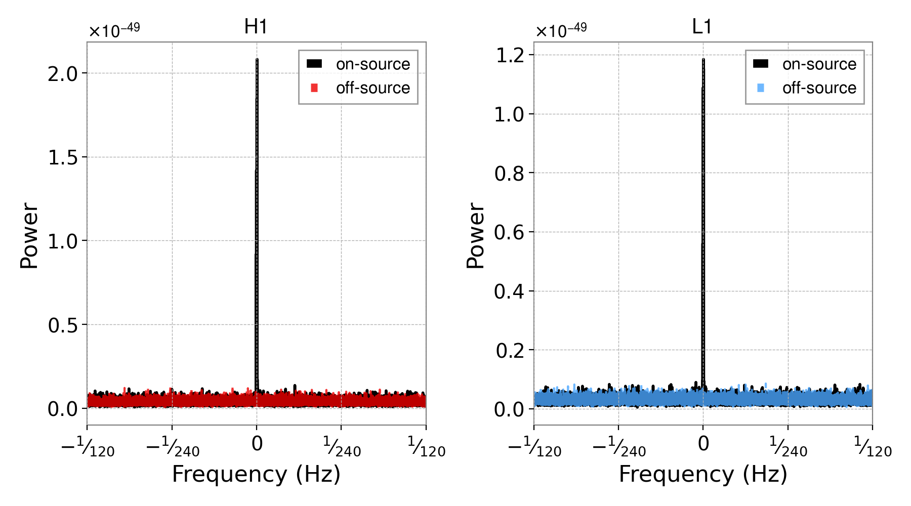
It is obvious from these that the strong hardware injection signal has been wiped out as a result of heterodyning using the wrong sky position.

The posterior probability distributions on the signal parameters, for the joint H1 and L1 analysis, can be plotted with:

import os

from cwinpy.info import HW_INJ
from cwinpy.plot import Plot

resdir = "results"

onsource = "JPULSAR03"
offsource = "JPULSAR03A"
pulnum = 3

for title, pulsar in zip(["on-source", "off-source"], [onsource, offsource]):
    resfile = os.path.join(resdir, pulsar, f"cwinpy_pe_H1L1_{pulsar}_result.hdf5")

    p = Plot(
        resfile,
        parameters=["h0", "iota", "phi0", "psi"],
        plottype="corner",
        pulsar=(HW_INJ["O1"]["hw_inj_files"][pulnum] if pulsar == "JPULSAR03" else None),
    )

    fig = p.plot()
    p.fig.suptitle(f"{title}")
    p.save(f"{pulsar}_H1L1_plot.png", dpi=200)
    p.fig.close()

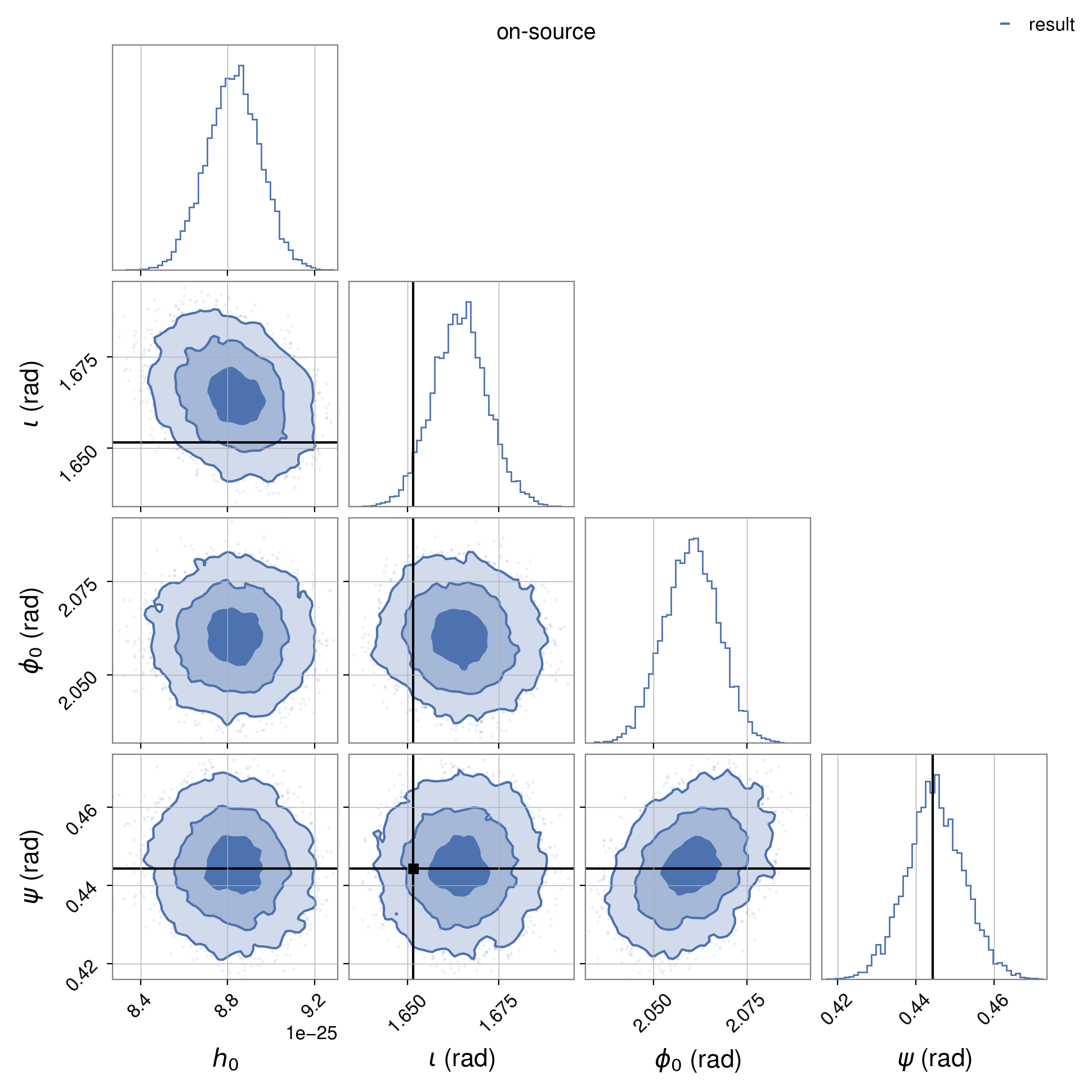
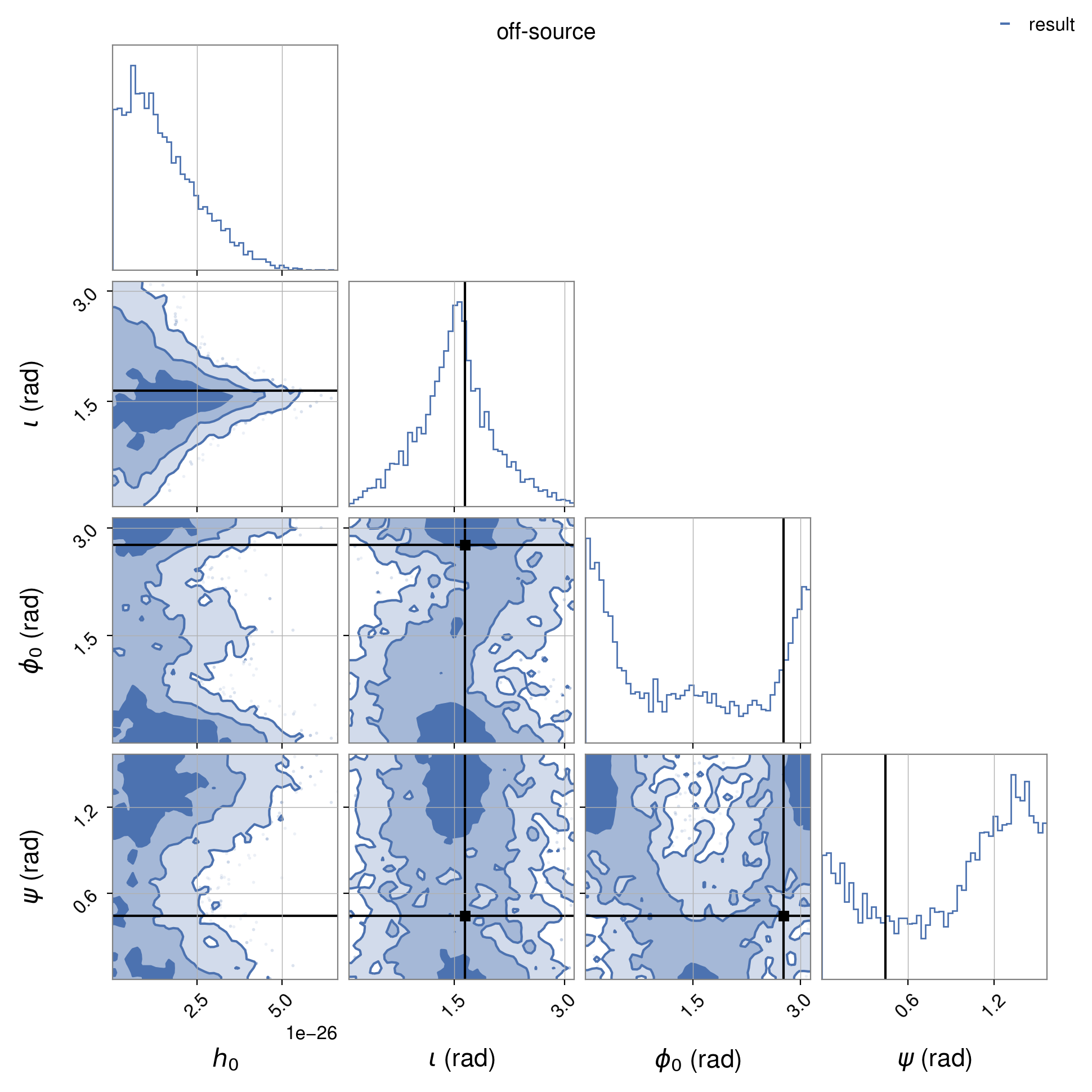
where the left image shows the “on-source” posteriors and the right the “off-source” (aka sky-shifted) posteriors.

Odds distribution

The distribution of odds values can be plotted in a variety of different ways using the skyshift_results() function. This can either plot the distribution in histogram form or on ths sky (if the healpy package is installed more options are available). skyshift_results() will calculate the odds using the results_odds() function for all the results produced by the sky-shift pipeline. As there are two detectors in this analysis, we can use the “coherent versus incoherent” odds as a way to assess the significance of the hardware injection signal.

A histogram of the background, sky-shifted, odds, can be plotted with the odds of on-source sky position shown as a dashed vertical line, using (from the skyshift directory):

from cwinpy.info import HW_INJ
from cwinpy.knope.skyshift import skyshift_results

s, t, fig = skyshift_results(
    "pulsars",
    HW_INJ["O1"]["hw_inj_files"][3],  # location of parameter file for hardware injection 03
    "results",
    plot="hist",
)

fig.show()

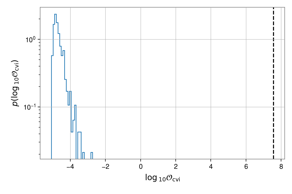
By default, this shows the “coherent versus incoherent” odds and uses a logarithmic scale for the y-axis. The s variable will hold a 3x500 array containing the right ascension, declination and odds for each sky-shifted source, while t will be tuple of these values for the on-source location. These can be passed to skyshift_results() rather than using the results directories if wanted to make further plots.

For example, we can plot the complementary cumulative distribution function (aka the survival function) and include a fit to a gamma distribution, with:

_, _, fig = skyshift_results(s, t, plot="invcdf", dist="gamma")
fig.show()

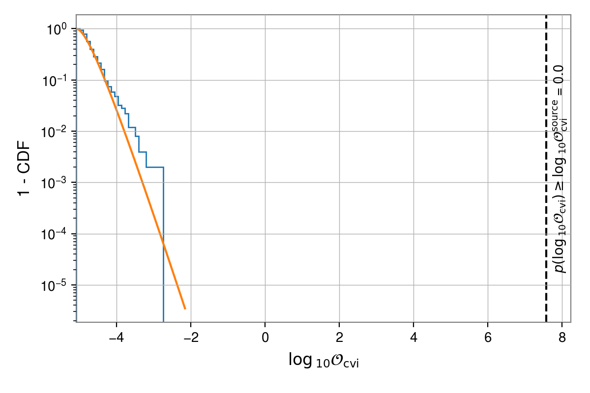
The plot displays the probability of the background producing an odds value equal to or greater than that from the on-source location. In this case that probability is essentially zero. However, it is worth noting that the background distribution appears to diverge from a gamma distribution in the tail.

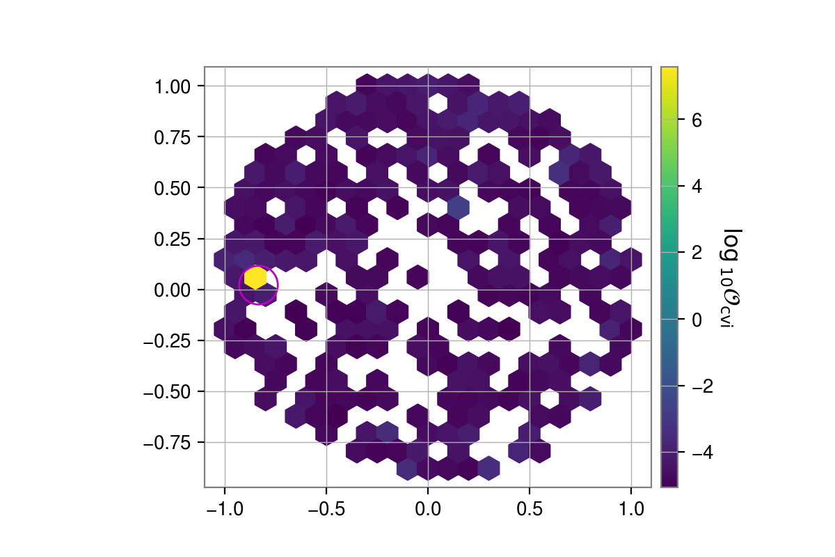
Sky distribution

The skyshift_results() function can also be used to show the distribution of odds values over the sky. If you do not have healpy installed, you can plot this using a matplotlib.pyplot.hexbin() plot, assuming s and t have already been produced as above with:

_, _, fig = skyshift_results(s, t, plot="hexbin")
fig.show()

If you have healpy installed you can plot “hammer”, “lambert”, “mollweide”, “cart”, or “aitoff” projection plots, e.g.,

_, _, fig = skyshift_results(s, t, plot="mollweide")
fig.show()

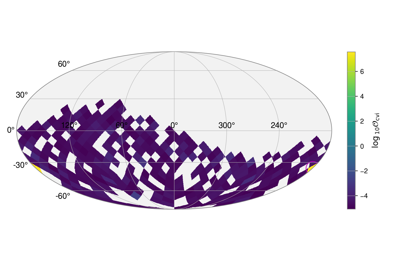
This shows how only half the sky is covered when generating the sky-shifted positions.

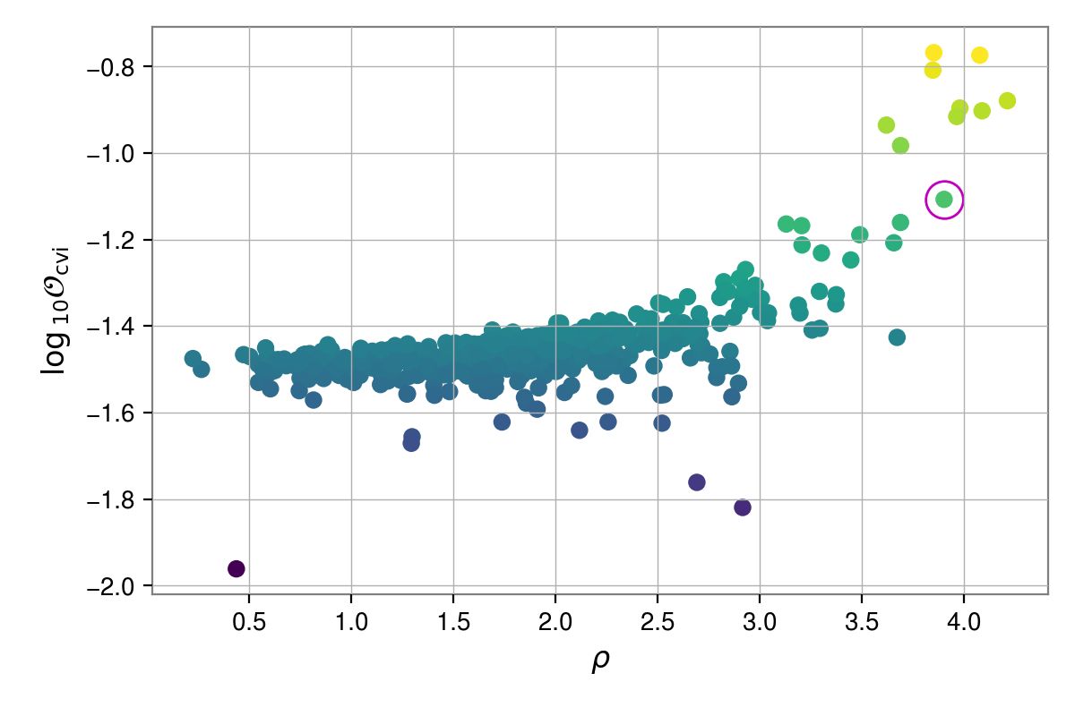
Odds versus signal-to-noise ratio

It can be useful to compare how the odds for each sky location are correlated with the recovered signal-to-noise ratio (SNR). This can be done using the plot_snr_vs_odds() function, which makes use of the optimal_snr() function. This will find the maximum a-posteriori, or maximum likelihood, sample from the parameter estimation for each sky location and calculate the optimal matched filter signal-to-noise ratio of a signal with those parameters. The plot_snr_vs_odds() can take in the heterodyned data directory and parameter estimation directory and compute odds and SNR itself, but below we will assume you use the results_odds() and optimal_snr() functions to given values that can be reused.

from cwinpy.pe.peutils import optimal_snr, plot_snr_vs_odds, results_odds

# get dictionary of odds ratios
odds = results_odds("results", oddstype="cvi")

# get SNRs (this may take some time, so save the output if you want to re-use it!)
snrs = optimal_snr("results", "stage2")

# extract the coherent H1-L1 SNRs
snrsjoint = {p: snrs[p]["H1L1"] for p in snrs}

# plot the on-source values
fig, ax = plot_snr_vs_odds(snrsjoint, odds, oddstype="cvi", scatterc="odds")

# highlight on-source value
ax.plot(snrsjoint["JPULSAR03"], odds["JPULSAR03"], marker="o", c="m", ms=15, mfc="none")

fig.show()

Note

When you have lots of sky-shifts the optimal_snr() function can take 10s of minutes to compute, so you will have to be patient!

Example: analysis outlier

In the search for gravitational-wave signals from pulsars using LIGO O1 data [6], the coherent versus incoherent signal odds for pulsar J1932+17 was an outlier when compared to these for the rest of the pulsars in the search sample. The sky-shifting method can be used to assess the significance of the outlier. In this case, as in [3], a log-uniform prior will be used on the gravitational-wave amplitude \(h_0\) (this is the uninformative Jeffreys prior for a scale parameter such as \(h_0\)), and therefore a configuration file must be used to set up the cwinpy_skyshift_pipeline rather than just using the “quick setup” options. The following configuration file, called outlier.ini, is used to run on O1 data for both LIGO detectors:

[run]
basedir = /home/matthew.pitkin/O1skyshift

[heterodyne_job]
accounting_group = aluk.dev.o1.cw.targeted.bayesian
accounting_group_user = matthew.pitkin

[heterodyne]
detectors = ['H1', 'L1']
starttimes = {'H1': 1126051217, 'L1': 1126051217}
endtimes = {'H1': 1137254417, 'L1': 1137254417}
frametypes = {'H1': 'H1_LOSC_16_V1', 'L1': 'L1_LOSC_16_V1'}
host = datafind.gwosc.org
channels = {'H1': 'H1:GWOSC-16KHZ_R1_STRAIN', 'L1': 'L1:GWOSC-16KHZ_R1_STRAIN'}
includeflags = {'H1': 'H1_CBC_CAT1', 'L1': 'L1_CBC_CAT1'}
excludeflags = {'H1': 'H1_NO_CW_HW_INJ', 'L1': 'L1_NO_CW_HW_INJ'}
overwrite = False
joblength = 86400

[merge]
remove = True
overwrite = True

[pe]
priors = /home/matthew.pitkin/O1skyshift/prior.txt

[ephemerides]
pulsarfiles = /home/matthew.pitkin/O1skyshift/J1932+17.par

which points to a prior.txt file containing:

h0 = LogUniform(minimum=1e-28, maximum=1.0e-21, name='h0', latex_label='$h_0$')
phi0 = Uniform(minimum=0.0, maximum=3.141592653589793, name='phi0', latex_label='$\phi_0$', unit='rad')
iota = Sine(minimum=0.0, maximum=3.141592653589793, name='iota', latex_label='$\iota$, unit='rad')
psi = Uniform(minimum=0.0, maximum=1.5707963267948966, name='psi', latex_label='$\psi$, unit='rad')

and a pulsar parameter file, as used by the O1 analysis based on observations from the Jodrell Bank Observatory, containing:

PSRJ	       J1932+17
RAJ            19:32:07.1674282          1  0.01023320381669795939   
DECJ           +17:56:18.70142           1  0.25231198765634132427   
F0             23.905550847651064273     1  0.00000000082758861857   
F1             -1.4458267504087269662e-15    6.7521640918638115878e-16
PEPOCH         56803.000211785492581       
POSEPOCH       56803.000211785492581
BINARY         ELL1
PB             41.507985998762112295     1  0.00000898573888192338   
A1             68.859148021929869263     1  0.00030720578073581612   
TASC           56765.946209275262305     1  0.00011436348933596476   
EPS1           -0.0001969460108668249454 1  0.00000737922338307618   
EPS2           0.00014522453787412931602 1  0.00000762676141481106   
UNITS          TCB
EPHEM          DE405

The analysis was the set up to run 500 sky-shifts with:

cwinpy_skyshift_pipeline --nshifts 500 outlier.ini

When using a configuration file the HTCondor jobs do not get automatically submitted unless specified in the file. Therefore, in this case the jobs were subsequently submitted using:

condor_submit_dag submit/cwinpy_skyshift.dag

As in the previous example, we can plot the distribution of odds values. To get a histogram with the

from cwinpy.knope.skyshift import skyshift_results

s, t, fig = skyshift_results(
    "pulsars",
    "J1932+17.par",
    "results",
    plot="invcdf",
    kde=True,
)
fig.show()

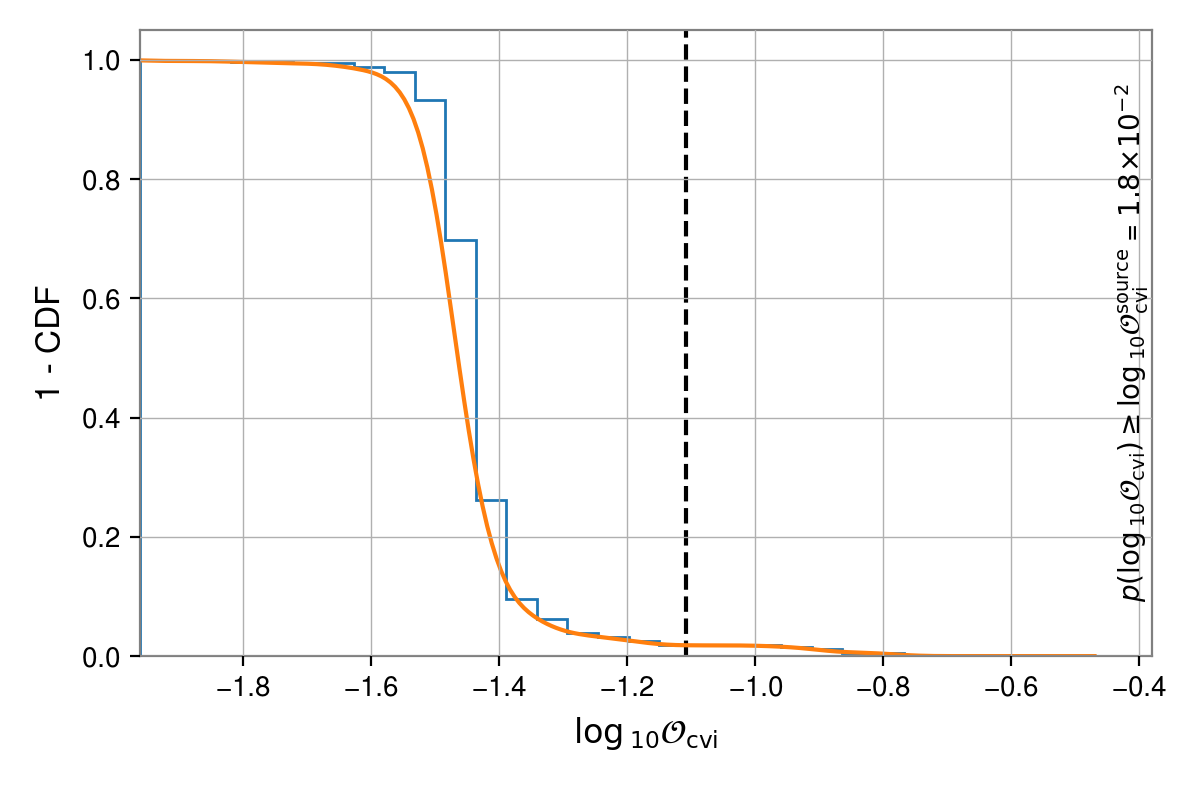
This overplots a kernel density estimate of the distribution (the gamma distribution used above does not provide a good fit in this case). It can be seen that despite the on-source value being an outlier, it is still within the distribution of background values and there are in fact larger odds in the background. The background distrbution suggests that there is about a 2% chance of getting an odds value equal or higher to the on-source value. In a search for hundreds of pulsars it would therefore be unsurprising to find such an outlier.

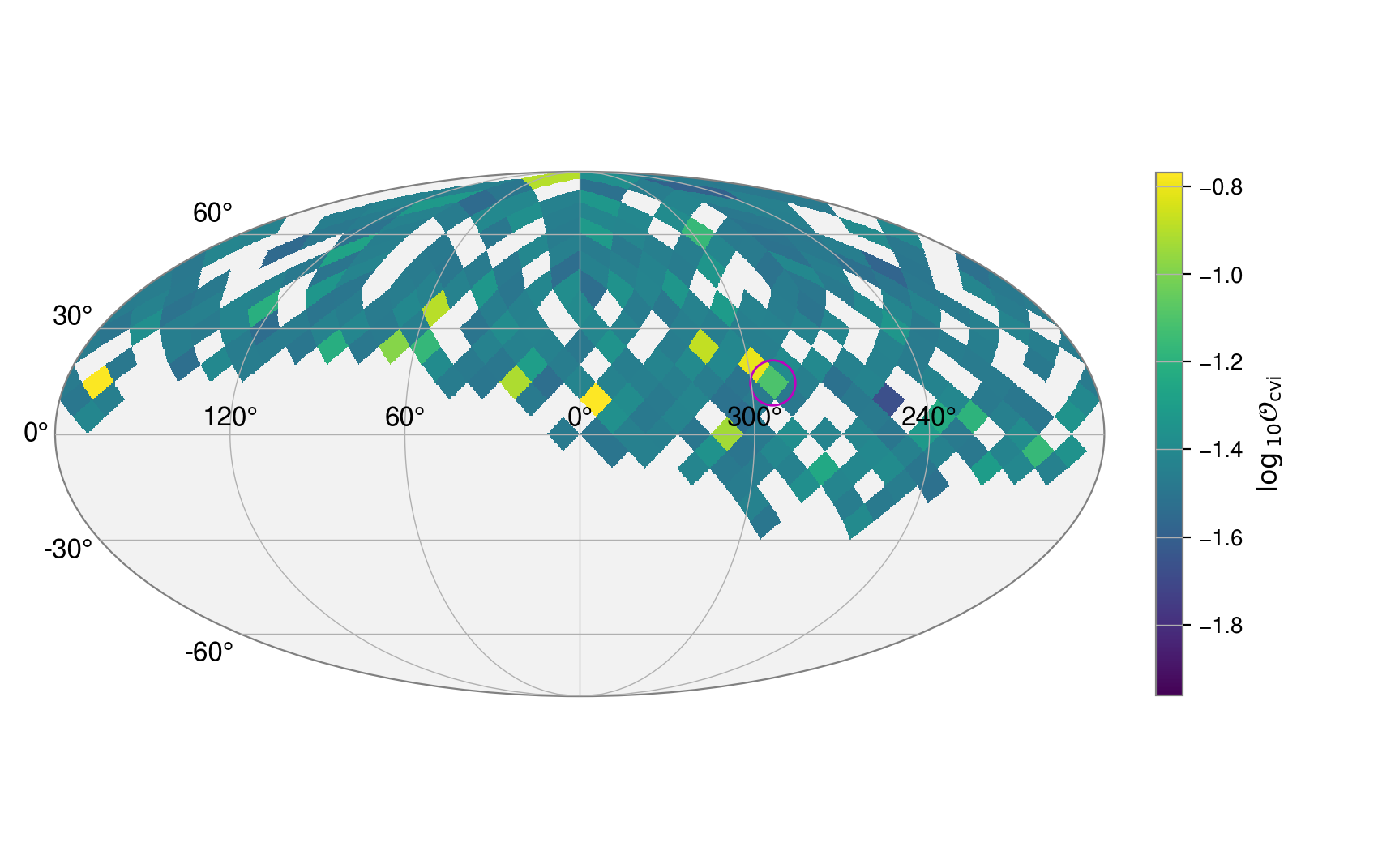
We can see how these odds values are distributed on the sky with:

_, _, fig = skyshift_results(s, t, plot="mollweide")

fig.show()

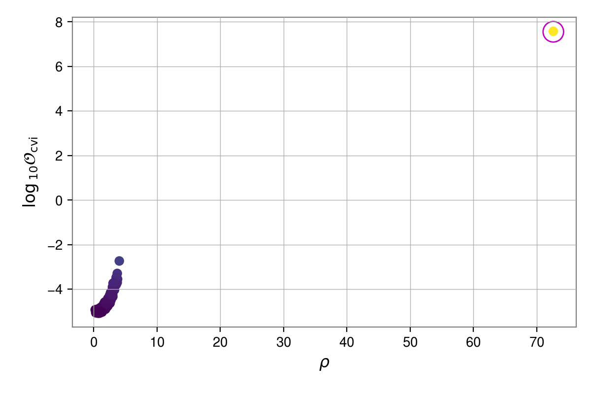
As in the previous example, we can look at the distribution of odds values plotted against the recovered signal-to-noise ratios. As above, we can calculate the SNRs using the (default) maximum a-posteriori sample:

from cwinpy.pe.peutils import optimal_snr, plot_snr_vs_odds, results_odds

oddsoutlier = results_odds("results", oddstype="cvi")
snrsoutlier = optimal_snr("results", "stage2")

snrsjoint = {p: snrsoutlier[p]["H1L1"] for p in snrsoutlier}
fig, ax = plot_snr_vs_odds(snrsjoint, oddsoutliers, oddstype="cvi", scatterc="odds", xscale="log")

# highlight on-source value
ax.plot(snrsjoint["J1932+17"], oddsoutliers["J1932+17"], marker="o", c="m", ms=15, mfc="none")

fig.show()

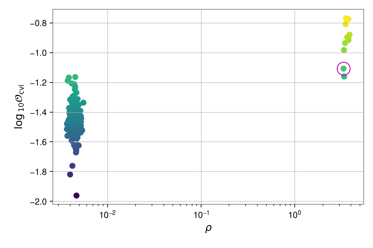
In the above plots, we’ve used a log-scale for the SNR axis due to the odd-looking SNR distribution. This SNR distribution is a product of using the log-uniform prior on the signal amplitude \(h_0\), causing most of the maximum a-posteriori values to be peaked close to zero. Even so, we see that the outlier signal is within a cluster of cases with SNR values above around 3, although it is not a unique outlier. We can instead switch to plotting the SNR generated using the maximum likelihood sample to give:

snrsoutliermaxL = optimal_snr("results", "stage2", which="likelihood")
snrsjoint = {p: snrsoutlier[p]["H1L1"] for p in snrsoutliermaxL}
fig, ax = plot_snr_vs_odds(snrsjoint, oddsoutliers, oddstype="cvi", scatterc="odds", xscale="log")

# highlight on-source value
ax.plot(snrsjoint["J1932+17"], oddsoutliers["J1932+17"], marker="o", c="m", ms=15, mfc="none")

fig.show()

Sky-shifting API

skyshift_pipeline(**kwargs)

Run skyshift pipeline within Python. This will create a HTCondor DAG for consecutively running a cwinpy_heterodyne and multiple cwinpy_pe instances on a computer cluster. Optional parameters that can be used instead of a configuration file (for “quick setup”) are given in the “Other parameters” section.

Parameters:

• config (str) – A configuration file, or configparser:ConfigParser object, for the analysis.

• nshifts (int) – The number of random sky-shifts to perform. The default will be 1000. These will be drawn from the same ecliptic hemisphere as the source.

• exclusion (float) – The exclusion region around the source’s actual sky location and any sky shift locations.

• overlap (float) – Provide a maximum allowed fractional overlap (e.g., 0.01 for a maximum 1% overlap) between the signal model at the true position and any of the sky-shifted position. If not given, this check will not be performed. If given, this check will be used in addition to the exclusion region check. Note: this does not check the overlap between each sky-shifted position, so some correlated sky-shifts may be present.

Other Parameters:

• run (str) – The name of an observing run for which open data exists, which will be heterodyned, e.g., “O1”.

• detector (str, list) – The detector, or list of detectors, for which the data will be heterodyned. If not set then all detectors available for a given run will be used.

• samplerate (str:) – Select the sample rate of the data to use. This can either be 4k or 16k for data sampled at 4096 or 16384 Hz, respectively. The default is 4k, except if running on hardware injections for O1 or later, for which 16k will be used due to being required for the highest frequency source. For the S5 and S6 runs only 4k data is available from GWOSC, so if 16k is chosen it will be ignored.

• pulsar (str) – The path to a TEMPO(2)-style pulsar parameter file to heterodyne. If a pulsar name is given instead of a parameter file then an attempt will be made to find the pulsar’s ephemeris from the ATNF pulsar catalogue, which will then be used.

• osg (bool) – Set this to True to run on the Open Science Grid rather than a local computer cluster.

• output (str) – The base location for outputting the heterodyned data and parameter estimation results. By default the current directory will be used. Within this directory, a subdirectory called “skyshift” will be created with subdirectories for each detector and for the result also created.

• joblength (int) – The length of data (in seconds) into which to split the individual heterodyne jobs. By default this is set to 86400, i.e., one day. If this is set to 0, then the whole dataset is treated as a single job.

• accounting_group (str) – For LVK users this sets the computing accounting group tag.

• usetempo2 (bool) – Set this flag to use Tempo2 (if installed) for calculating the signal phase evolution for the heterodyne rather than the default LALSuite functions.

• incoherent (bool) – If running with multiple detectors, set this flag to analyse each of them independently rather than coherently combining the data from all detectors. A coherent analysis and an incoherent analysis is run by default.

Returns:

An object containing a pycondor pycondor.Dagman object.

Return type:

dag

skyshift_pipeline_cli(**kwargs)

Entry point to cwinpy_skyshift_pipeline script. This just calls cwinpy.knope.skyshift_pipeline(), but does not return any objects.

skyshift_results(shift, orig, resdir=None, oddstype='cvi', scale='log10', plot=False, kde=False, dist=None, yscale='log', **kwargs)

Using the output of the cwinpy_skyshift_pipeline, generate the Bayesian odds statistic for each shifted location and the original location. These can also be plotted if requested, which will additionally return a Figure object containing the plot.

If you already have the output of this function and just want to (re)produce a plot, then you can instead pass in the results from the previous call and use those.

Parameters:

• shift (str, array) – If generating the results, this should be the directory containing the pulsar parameter (.par) files for all the sky-shifted locations. If using pre-generated results, i.e., to (re)produce a plot, then this should be the Nx3 array containing the right ascension, declination and odds for all the sky-shifted sources.

• orig (str, tuple) – If generating the results, this should be the pulsar parameter (.par) file containing the original un-shifted location. If using pre-generated results, then this should be a length 3 array containing the right ascension, declination and odds to the true source.

• resdir (str) – The directory containing the parameter estimation outputs for each sky-shifted location.

• oddstype (str) – The odds type used by results_odds(). Defaults to "cvi".

• scale (str) – The odds scale used by results_odds(). Defaults to "log10".

• plot (str, bool) – If plot is given as "hist" a histogram of the distribution of sky-shifted odds values will be produced; if “invcdf”, then it will plot the distribution (1 - CDF); if "hexbin", then a matplotlib.pyplot.hexbin() plot will be produced using the sky positions converted into a cartesian coordinate system and the maximum odds in each bin; if healpy is installed then the healpy.newvisufunc.projview() function will be used if any of the following arguments are given "hammer", "lambert", "mollweide", "cart", or "aitoff", which will plot the maximum odds in each HEALPix pixel. This defaults to False, i.e., no plot will be produced.

• plotkwargs (dict) – If making a plot, and further keyword arguments required for the plotting function can be passed using this dictionary.

• kde (bool) – If plotting a histogram plot and this is True, a KDE of the distribution will also be added using the scipy.stats.gaussian_kde function. The probability of getting a value greater than the true sky position’s odds based on the KDE will be added to the plot. If the dist argument is given then the KDE will be ignored and the gamma distribution plotted instead.

• kdekwargs (dict) – If plotting a KDE, any keyword arguments can be passed using this dictionary.

• dist (str) – If plotting the histogram (and not plotting a KDE) then a fit to that histogram can also be added based on the name of the distribution given by this argument. Currently, the value here can either be "gamma" (using scipy.stats.gamma) or "gumbel" (using scipy.stats.gumbel_r), for whi a best fit of the given distribution will be plotted. The probability of getting a value from that distribution greater than the true sky position’s odds will be added to the plot.

• yscale (str) – The scaling on the y-axis of a histogram or inverse CDF plot will default to a log scale. To set it to a linear scale set this argument to "linear".

Returns:

• shiftodds (array) – A numpy.ndarray() containing the right ascension, declination and odds value for all sky-shifted locations.

• trueodds (tuple) – A tuple containing the right ascension, declination and odds for the original un-shifted location.

Sky-shifting references

[1]

D. Davis et al, CQG, 38, 135014 (2021).

[2]

P. Covas et al, PRD, 97, 082002 (2018).

[3] (1,2)

M. Isi, S. Mastrogiovanni, M. Pitkin & O. J. Piccinni, PRD, 102, 123027 (2020).

[4]

S. A. Usman et al, CQG, 33, 215004 (2016).

[5]

M. Pitkin, M. Isi, J. Veitch & G. Woan, arXiv:1705.08978v1 (2017).

[6]

B. P. Abbott et al, ApJ, 839, 12 (2017).