Simulating a signal

Here we describe the HeterodynedCWSimulator class for simulating a signal from a continuous wave source after application of a heterodyne as described in Equations 7 and 8 of [1].

When generating the signal using the model() method, the default is to assume that the phase evolution used in the heterodyne exactly matches the signal’s phase evolution and that emission is from the \(l=m=2\) quadrupole mode (a triaxial source emitting at twice the rotation frequency), i.e., the \(\Delta\phi\) term in Equations 8 of [1] is zero. If the file/object that provides the signal parameters contains parameters for non-tensorial polarisation modes (i.e., if assuming emission is not purely as given by general relativity; see Table 6 of [1] for the names of the required parameters) then those polarisations will be included in the signal (e.g., Equation 11 of [1]), otherwise general relativity will be assumed and only the “+” and “×” polarisations included.

The model() method can also generate model amplitude coefficients for use in a “pre-summed” likelihood function, as described in Appendix C and Equations C8 and C12 of [1], by passing the outputampcoeffs argument as True. For a GR signal this means two complex amplitude values get returned, while for non-GR signals six complex amplitudes are returned.

The signal model at the rotation frequency, i.e., from the \(l=2,m=1\) mode, can be set by passing freqfactor=1.0 as an argument to model(). This requires that the file/object containing the source parameters has the \(C_{21}\) and \(\Phi_{21}\) parameters defined as given in Equation 7 of [1].

Note

If generating a simulated signal in IPython or a Jupyter notebook, creating an instance of this class can be very slow (taking minutes compared to a fraction of a second), due to redirections of stdout/stderr in the SWIG-wrapped LIGOTimeGPS class. To avoid this the call to HeterodynedCWSimulator should be either done within a context manager, e.g.,:

import lal

with lal.no_swig_redirect_standard_output_error():
      sim = HeterodyneCWSimulator(...)

or by globally disabling redirection with:

import lal

lal.swig_redirect_standard_output_error(True)

sim = HeterodyneCWSimulator(...)

Phase offset signal

The model() method can also be used to generate a signal that is offset, in terms of its phase evolution, from the heterodyne phase. This can be used to simulate cases where the heterodyned was not performed with an identical phase evolution to the signal (due to differences between the source rotational/binary parameters). The pulsar parameter file/object passed when constructing a HeterodynedCWSimulator object is assumed to contain the parameters for the heterodyne phase model, while model() can be passed an “updated” file/object containing potentially different (phase) parameters that are the “true” source parameters using the newpar argument (and updateX arguments for defining which components of the phase evolution need updating compared to the heterodyne values). The difference in phase, as calculated using Equation 10 of [1], will then be used when generating the signal.

Using Tempo2

By default, the phase difference evolution will be calculated using functions within LALSuite, which has its own routines for calculating the solar system and binary system delay terms. However, if the Tempo2 pulsar timing software [2], and the libstempo Python wrapper for this, are installed, then Tempo2 can instead be used for the generation of the phase evolution. This is done by setting the usetempo2 argument to model() to True.

Note

If using Tempo2 you cannot use the updateX keyword arguments to specify whether or not to recalculate a component of the phase model. All components will be regenerated if present.

Examples

An example usage to generate the complex heterodyned signal time series is:

from cwinpy.signal import HeterodynedCWSimulator
from cwinpy import PulsarParameters
from astropy.time import Time
from astropy.coordinates import SkyCoord
import numpy as np

# set the pulsar parameters
par = PulsarParameters()
pos = SkyCoord("01:23:34.5 -45:01:23.4", unit=("hourangle", "deg"))
par["PSRJ"] = "J0123-4501"
par["RAJ"] = pos.ra.rad
par["DECJ"] = pos.dec.rad
par["F"] = [123.456789, -9.87654321e-12]  # frequency and first derivative
par["PEPOCH"] = Time(58000, format="mjd", scale="tt").gps  # frequency epoch
par["H0"] = 5.6e-26     # GW amplitude
par["COSIOTA"] = -0.2   # cosine of inclination angle
par["PSI"] = 0.4        # polarization angle (rads)
par["PHI0"] = 2.3       # initial phase (rads)

# set the GPS times of the data
times = np.arange(1000000000.0, 1000086400.0, 3600, dtype=np.float128)

# set the detector
det = "H1"  # the LIGO Hanford Observatory

# create the HeterodynedCWSimulator object
het = HeterodynedCWSimulator(par, det, times=times)

# get the model complex strain time series
model = het.model()

Note

If you have a pulsar parameter file you do not need to create a PulsarParameters object, you can just pass the path of that file, e.g.,

par = "J0537-6910.par"
het = HeterodynedCWSimulator(par, det, times=times)

An example (showing both use of the default phase evolution calculation and that using Tempo2) of getting the time series for a signal that has phase parameters that are not identical to the heterodyned parameters would be:

from cwinpy.signal import HeterodynedCWSimulator
from cwinpy import PulsarParameters
from astropy.time import Time
from astropy.coordinates import SkyCoord
from copy import deepcopy
import numpy as np

# set the "heterodyne" pulsar parameters
par = PulsarParameters()
pos = SkyCoord("01:23:34.5 -45:01:23.4", unit=("hourangle", "deg"))
par["PSRJ"] = "J0123-4501"
par["RAJ"] = pos.ra.rad
par["DECJ"] = pos.dec.rad
par["F"] = [123.4567, -9.876e-12]  # frequency and first derivative
par["PEPOCH"] = Time(58000, format="mjd", scale="tt").gps  # frequency epoch
par["H0"] = 5.6e-26     # GW amplitude
par["COSIOTA"] = -0.2   # cosine of inclination angle
par["PSI"] = 0.4        # polarization angle (rads)
par["PHI0"] = 2.3       # initial phase (rads)

# set the times
times = np.arange(1000000000.0, 1000086400.0, 600, dtype=np.float128)

# set the detector
det = "H1"  # the LIGO Hanford Observatory

# create the HeterodynedCWSimulator object
het = HeterodynedCWSimulator(par, det, times=times)

# set the updated parameters
parupdate = deepcopy(par)
parupdate["RAJ"] = pos.ra.rad + 0.001
parupdate["DECJ"] = pos.dec.rad - 0.001
parupdate["F"] = [123.456789, -9.87654321e-12]  # different frequency and first derivative

# get the model complex strain time series
model = het.model(parupdate, updateSSB=True)

# do the same but using Tempo2
hettempo2 = HeterodynedCWSimulator(par, det, times=times, usetempo2=True)
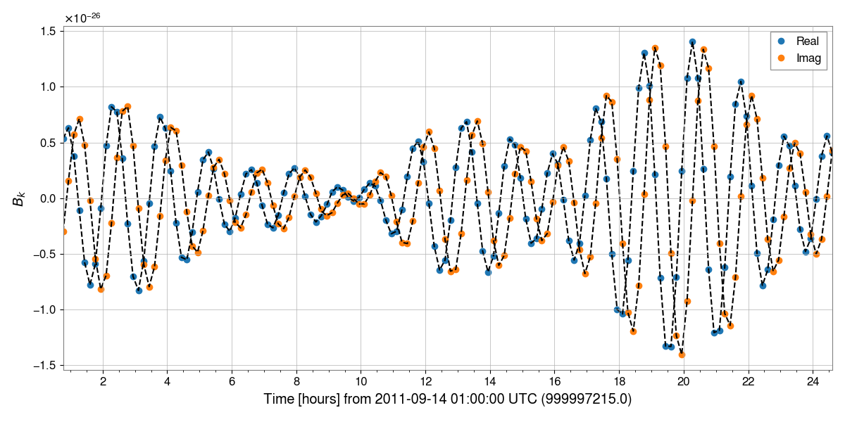
modeltempo2 = hettempo2.model(parupdate)

Overplotting these (the Tempo2 version is shown as black dashed lines) we see:

from cwinpy import HeterodynedData

hetdata = HeterodynedData(model, times=times, detector=det, par=parupdate)
fig = hetdata.plot(which="both")
ax = fig.gca()

# over plot Tempo2 version
ax.plot(times, modeltempo2.real, "k--")
ax.plot(times, modeltempo2.imag, "k--")
fig.tight_layout()

Note

For signals from sources in binary systems there will be a phase offset between signals heterodyned using the default LALSuite functions and those using Tempo2. This offset is not present for non-binary sources. In general this is not problematic, but if using Tempo2 it will mean that the recovered initial phase will not be consistent with the expected value.

In this example using Tempo2 is several hundred times slower, but still runs in about a hundred ms rather than a couple of hundred μs.

Signal API

class HeterodynedCWSimulator(par, det, times=None, earth_ephem=None, sun_ephem=None, ephem='DE405', units='TCB', usetempo2=False, t0=None, dt=None)

Bases: object

A class to simulate strain data for a continuous gravitational-wave signal after the data has been heterodyned, i.e., after multiplying the data by a complex phase vector. This uses the Equations 7 and 8 from [1] accessed via the XLALHeterodynedPulsarGetModel() function.

Parameters:

• par (str, PulsarParameters) – A Tempo-style text file, or a PulsarParameters object, containing the parameters for the source, in particular the phase parameters at which the data is “heterodyned”.

• det (str) – The name of a gravitational-wave detector.

• times (array_like) – An array of GPS times at which to calculate the heterodyned strain.

• t0 (float) – A time epoch in GPS seconds at which to calculate the detector response function. If not given and times is set, then the first value of times will be used.

• dt (int, float) – The time steps (in seconds) in the data over which to average the detector response. If not given and times is set, then the time difference between the first two values in times will be used.

• earth_ephem (str) – A file containing the LALSuite-style Earth ephemeris information. If not set then a default file will be used.

• sun_ephem (str) – A file containing the LALSuite-style Sun ephemeris information. If not set then a default file will be used.

• ephem (str) – The solar system ephemeris system to use for the Earth and Sun ephemeris, i.e., "DE200", "DE405", "DE421", or "DE430". By default the EPHEM value from the supplied par will be used, but if not found, and if this value is not set, it will default to "DE405".

• units (str) – The time system used, i.e., "TDB" or "TCB". By default the UNITS value from the par will be used, but if not found, and if this value is not set, it will (like TEMPO2) default to "TCB".

• usetempo2 (bool) – Set to True to use TEMPO2, via libstempo, for calculating the phase of the signal. To use libstempo must be installed. If using TEMPO2 the Earth, Sun and time ephemerides, and the ephem and units arguments are not required. Information on the correct ephemeris will all be calculated internally by TEMPO2 using the information from the pulsar parameter file.

model(newpar=None, updateSSB=False, updateBSB=False, updateglphase=False, updatefitwaves=False, freqfactor=2.0, outputampcoeffs=False, roq=False)

Compute the heterodyned strain model using XLALHeterodynedPulsarGetModel().

Parameters:

• newpar (str, PulsarParameters) – A text parameter file, or PulsarParameters object, containing a set of parameter at which to calculate the strain model. If this is None then the “heterodyne” parameters are used.

• updateSSB (bool) – Set to True to update the solar system barycentring time delays compared to those used in heterodyning, i.e., if the newpar contains updated positional parameters.

• updateBSB (bool) – Set to True to update the binary system barycentring time delays compared to those used in heterodying, i.e., if the newpar contains updated binary system parameters

• updateglphase (bool) – Set to True to update the pulsar glitch evolution compared to that used in heterodyning, i.e., if the newpar contains updated glitch parameters.

• updatefitwaves (bool) – Set to True to update the pulsar FITWAVES phase evolution (used to model strong red timing noise) compared to that used in heterodyning.

• freqfactor (int, float) – The factor by which the frequency evolution is multiplied for the source model. This defaults to 2 for emission from the \(l=m=2\) quadrupole mode.

• outputampcoeffs (bool) – If False (default) then the full complex time series of the signal (calculated at the time steps used when initialising the object) will be output. If True only two complex amplitudes (six for non-GR sources) will be output for use when a pre-summed signal model is being used - this should only be used if phase parameters are not being updated.

• roq (bool) – A boolean value to set to True if requiring the output for a ROQ model (NOT YET IMPLEMENTED).

Returns:

strain – A complex array containing the strain data

Return type:

array_like

property resp

Return the response function look-up table.

Signal references

[1] (1,2,3,4,5,6,7,8)

M. Pitkin, M. Isi, J. Veitch & G. Woan, arXiv:1705.08978v1 (2017).

[2]

G. B. Hobbs, R. T. Edwards, R. N. Manchester, MNRAS, 369, 2 (2006).