Reduced Order Quadrature

When performing Bayesian parameter estimation, it is often the case that calculating the likelihood function is the main computational expenses. This could be due to the likelihood being calculated for a large data set, or the source model being slow to evaluate, or a combination of both. Stochastic sampling methods often required hundreds of thousands or millions of likelihood evaluations to properly characterise the posterior probability distribution, so a slow likelihood means slow inference.

A method for speeding up the likelihood evaluation is to use Reduced Order Quadrature (ROQ) [1] [2] [3]. This works well if the source model has some strong correlations within the required parameter space. In such a case, a set of orthonormal basis vectors can be found that when linearly combined with appropriate weights gives an accurate representation of the original model anywhere in parameter space. The basis vectors can be precomputed before any inference and used to generate an interpolant for the model. If there are \(N\) basis vectors, the original model only needs to be calculated at \(N\) points to work out the weights for combining the basis vectors to reproduce the full model. If the original length of the data is \(M\) and \(N \ll M\) then there can be a significant speed up in calculating the model.

ROQ itself refers to a further neat trick that reduces the need to sum terms in the likelihood function over the full \(M\) values and instead only sum over \(N\) values. The basis vectors allow the construction of pre-calculated interpolants for the \((d \cdot m)\) and \((m \cdot m)\) terms in the likelihood (where \(d\) and \(m\) are the data and the model, respectively) that again only rely on the model being calculated at \(N\) values to accurately reconstruct the full terms.

There is, of course, some initial overhead to calculating the basis vectors, but this is often relatively small compared to the overall savings over the course of the full parameter estimation. There may also be cases where the parameter space is too uncorrelated (maybe just due to being too large) to mean that the number of basis vectors is less than the overall length of the data. In such cases, you can just revert back to calculating the full likelihood.

CWInPy uses the arby package for the generation of the reduced order model, reduced basis vectors and interpolants for the likelihood function components.

ROQ in CWInPy

Within CWInPy, if performing parameter estimation in the case where the heterodyne has been assumed to perfectly remove the signal’s phase evolution (i.e., no parameters that cause the phase to evolve, such as frequency or sky location parameters, are to be estimated) then the likelihood function is already efficient and uses pre-summed terms (see dot_products() and Appendix C of [4]). However, if the phase is potentially evolving (i.e., the observed electromagnetic pulse timing solution does not exactly match the gravitational-wave evolution and a residual phase evolution is left in the heterodyned data), and as such parameter estimation needs to be performed over some phase parameters (e.g., frequency) then these pre-summations cannot be done and each likelihood evaluation for different phase parameter values must re-calculate the model at all time stamps in the data. Along with the generally larger parameter space to explore, this will considerably slow down the inference.

While CWInPy’s likelihood evaluations will operate in this mode by default, in these cases it can be useful to instead use Reduced Order Quadrature to potentially help speed things up. There are several caveats to this, in particular, different frequency bins are highly uncorrelated, so it is unlikely that a small reduced basis set will be found if the frequency offset is many tens of frequency bins. Also, for the length of dataset often found in practice (of order a million data points over a year of observations), computer memory constraints may make it necessary to build the reduced basis on shorter blocks of data. Unlike the use of ROQs for parameter estimation with Compact Binary Coalescences [2], the same set of basis vectors cannot generally be used for different sources, so they need to be calculated individually for each source and dataset.

Usage

The usage of the ROQ likelihood can be specified by using keyword arguments to the cwinpy.pe.pe() functions, e.g.,

pe(
    ...
    roq=True,
    roq_kwargs={"ntraining": 5000, "greedy_tol": 1e-12},
)

where the roq_kwargs dictionary contains keywords for the GenerateROQ class.

These keywords can also be used in the cwinpy_pe, cwinpy_pe_pipeline, cwinpy_knope and cwinpy_knope_pipeline configuration files or APIs. For example, to use the ROQ likelihood a cwinpy_pe configuration file would contain:

roq = True
roq_kwargs = {'ntraining': 5000, 'greedy_tol': 1e-12}

Attention

There are several things to be aware of when using the ROQ likelihood:

1. When generating the reduced order model, a training set of ntraining models is produced. If this number is large and the data set is long, this can potentially run into computer memory constraints, due to the full matrix of training models needing to be stored in memory. To avoid this, the bbmaxlength keyword of the HeterodynedData class can be passed to ensure that the data is broken up into smaller chunks on which the model can be individually trained. This would be achieved through the data_kwargs keyword of cwinpy.pe.pe(), e.g., using

pe(
    ...
    roq=True,
    roq_kwargs={"ntraining": 5000, "greedy_tol": 1e-12},
    data_kwargs={"bbmaxlength": 10000},
)

if using cwinpy.pe.pe() directly, or

roq = True
roq_kwargs = {'ntraining': 5000, 'greedy_tol': 1e-12}
data_kwargs = {'bbmaxlength': 10000}

in a configuration file.

2. To give the reduced order model the best chance of producing a reduced basis that is not too large, it is best (if possible) to try and update the pulsar parameter file being used to have its epoch, i.e., the PEPOCH value, being at the start or the centre of the dataset that is being analysed. This may require updating frequencies, frequency derivatives and sky locations to that epoch, as applicable. This may be more necessary if using the ROQ likelihood for known pulsars with an older observation epoch, but should not be problematic if following up CW candidates from other wider parameter CW signal searches.

3. If wanting to use the ROQ as part of a pipeline running on multiple pulsars, you will most likely have to specify different prior files for each pulsar. This can be done by making sure that the priors option in the configuration file, or passed directly to cwinpy.pe.pe(), is either:

• the path to a directory that contains individual prior files for each pulsar, where the files are identified by containing the pulsar’s PSRJ name in the filename;

• a list of paths to individual prior files for each pulsar, where the files are identified by containing the pulsar’s PSRJ name in the filename;

• or, a dictionary with keys being the pulsar PSRJ names and values being paths to the prior file for that pulsar.

For example, the configuration file could contain:

priors = ['/home/user/parfiles/J0534+2200.prior', '/home/user/parfiles/J0835-4510.par']

# or alternatively (if the prior files are in the same directory)
priors = /home/user/parfiles

# or using a dictionary (if, say, the prior files do not contain the
# pulsar name in the file name)
priors = {'J0534+2200': '/home/user/parfiles/crab.prior', 'J0835-4510': '/home/user/parfiles/vela.par'}

ROQ comparison example

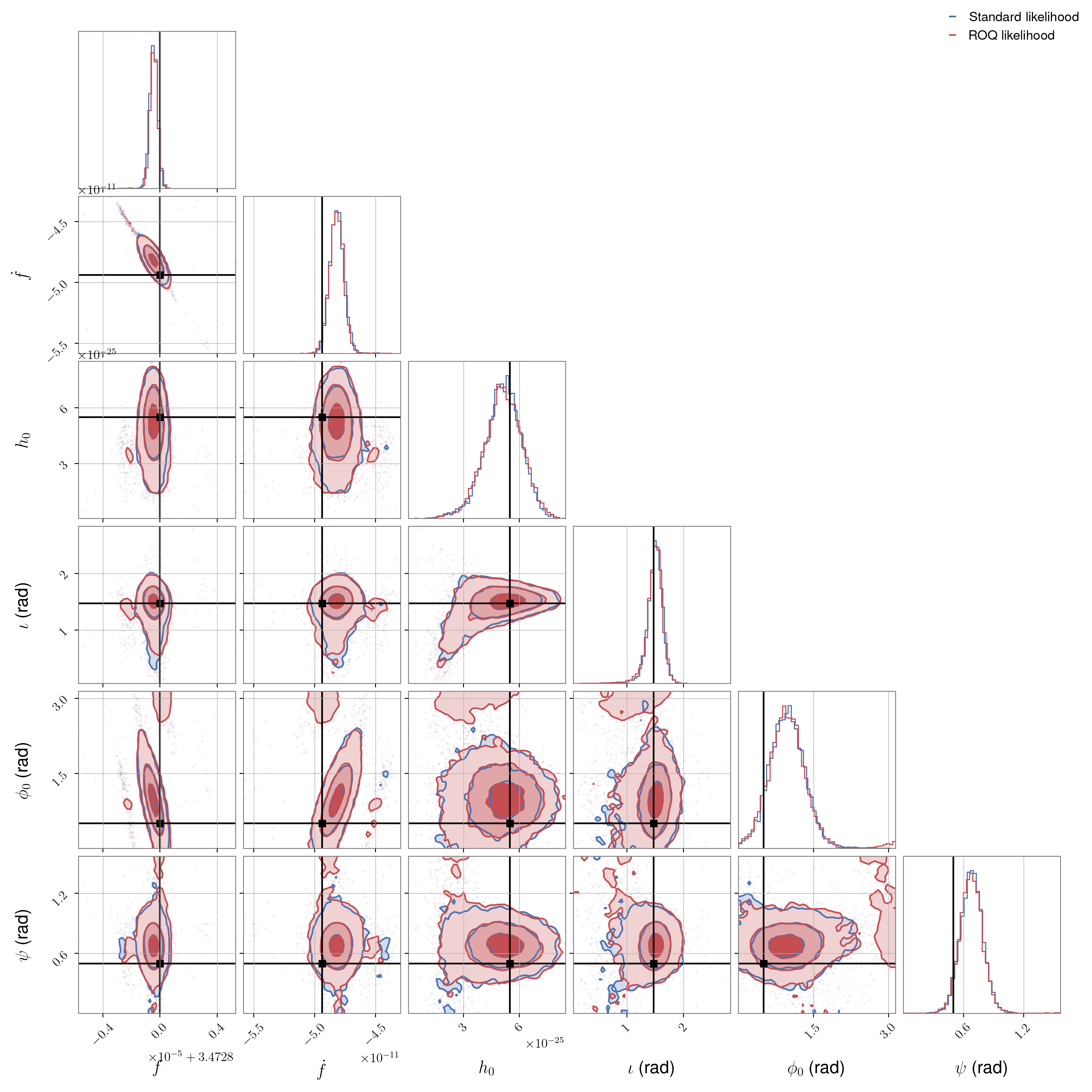
In a first example of using the ROQ likelihood, we will generate a simulated continuous signal and then purposely heterodyne it using frequency and frequency derivative parameters that are offset from the “true” values. We will then attempt to estimate the source parameters including the frequency and frequency derivative using (for comparison) both the standard likelihood and the ROQ likelihood. The script for this is shown below.

To view the code that generates the simulated signal click the hidden dropdown below.

Signal generation

import os
import shutil
import subprocess as sp

import numpy as np
from cwinpy.heterodyne import heterodyne
from cwinpy.plot import Plot
from cwinpy.utils import LAL_EPHEMERIS_URL, download_ephemeris_file

# generate some fake data using lalpulsar_Makefakedata_v5
mfd = shutil.which("lalpulsar_Makefakedata_v5")

fakedatadir = "fake_data"
fakedatadetector = "H1"
fakedatachannel = f"{fakedatadetector}:FAKE_DATA"

fakedatastart = 1000000000
fakedataduration = 864000

os.makedirs(fakedatadir, exist_ok=True)

fakedatabandwidth = 8  # Hz
sqrtSn = 2e-23  # noise amplitude spectral density
fakedataname = "FAKEDATA"

# create one pulsar to inject
fakepulsarpar = []

# requirements for Makefakedata pulsar input files
pulsarstr = """\
Alpha = {alpha}
Delta = {delta}
Freq = {f0}
f1dot = {f1}
f2dot = {f2}
refTime = {pepoch}
h0 = {h0}
cosi = {cosi}
psi = {psi}
phi0 = {phi0}
"""

# pulsar parameters
f0 = 6.9456 / 2.0  # source rotation frequency (Hz)
f1 = -9.87654e-11 / 2.0  # source rotational frequency derivative (Hz/s)
f2 = 2.34134e-18 / 2.0  # second frequency derivative (Hz/s^2)
alpha = 0.0  # source right ascension (rads)
delta = 0.5  # source declination (rads)
pepoch = 1000000000  # frequency epoch (GPS)

# GW parameters
h0 = 5.5e-25  # GW amplitude
phi0 = 1.0  # GW initial phase (rads)
iota = 1.47
cosiota = np.cos(iota)  # cosine of inclination angle
psi = 0.5  # GW polarisation angle (rads)

mfddic = {
    "alpha": alpha,
    "delta": delta,
    "f0": 2 * f0,
    "f1": 2 * f1,
    "f2": 2 * f2,
    "pepoch": pepoch,
    "h0": h0,
    "cosi": cosiota,
    "psi": psi,
    "phi0": phi0,
}

fakepulsarpar = PulsarParameters()
fakepulsarpar["PSRJ"] = "J0000+0000"
fakepulsarpar["H0"] = h0
fakepulsarpar["PHI0"] = phi0 / 2.0
fakepulsarpar["PSI"] = psi
fakepulsarpar["IOTA"] = iota
fakepulsarpar["F"] = [f0, f1, f2]
fakepulsarpar["RAJ"] = alpha
fakepulsarpar["DECJ"] = delta
fakepulsarpar["PEPOCH"] = pepoch
fakepulsarpar["EPHEM"] = "DE405"
fakepulsarpar["UNITS"] = "TDB"

fakepardir = "par_dir"
os.makedirs(fakepardir, exist_ok=True)
fakeparfile = os.path.join(fakepardir, "J0000+0000.par")
fakepulsarpar.pp_to_par(fakeparfile)

injfile = os.path.join(fakepardir, "inj.dat")
with open(injfile, "w") as fp:
    fp.write("[Pulsar 1]\n")
    fp.write(pulsarstr.format(**mfddic))
    fp.write("\n")

# set ephemeris files
efile = download_ephemeris_file(LAL_EPHEMERIS_URL.format("earth00-40-DE405.dat.gz"))
sfile = download_ephemeris_file(LAL_EPHEMERIS_URL.format("sun00-40-DE405.dat.gz"))

cmds = [
    "-F",
    fakedatadir,
    f"--outFrChannels={fakedatachannel}",
    "-I",
    fakedatadetector,
    "--sqrtSX={0:.1e}".format(sqrtSn),
    "-G",
    str(fakedatastart),
    f"--duration={fakedataduration}",
    f"--Band={fakedatabandwidth}",
    "--fmin",
    "0",
    f'--injectionSources="{injfile}"',
    f"--outLabel={fakedataname}",
    f'--ephemEarth="{efile}"',
    f'--ephemSun="{sfile}"',
    "--randSeed=1234",  # for reproducibility
]

# run makefakedata

import copy
import numpy as np
from bilby.core.prior import PriorDict, Sine, Uniform

from cwinpy.heterodyne import heterodyne
from cwinpy.parfile import PulsarParameters
from cwinpy.pe import pe
sp.run([mfd] + cmds)

# resolution
res = 1 / fakedataduration

# set priors for PE
priors = PriorDict()
priors["h0"] = Uniform(0, 1e-23, name="h0", latex_label="$h_0$")
priors["phi0"] = Uniform(0, np.pi, name="phi0", latex_label=r"$\phi_0$", unit="rad")
priors["psi"] = Uniform(0, np.pi / 2, name="psi", latex_label=r"$\psi$", unit="rad")
priors["iota"] = Sine(name="iota", latex_label=r"$\iota$")

priors["f0"] = Uniform(
    f0 - 5 * res, f0 + 5 * res, name="f0", latex_label=r"$f$", unit="Hz"
)
priors["f1"] = Uniform(
    f1 - 5 * res**2,
    f1 + 5 * res**2,
    name="f1",
    latex_label=r"$\dot{f}$",
    unit="Hz/s",
)

# perform heterodyne with f0 and f1 offset from true values
segments = [(fakedatastart, fakedatastart + fakedataduration)]

fulloutdir = os.path.join(fakedatadir, "heterodyne_output")

offsetpar = copy.deepcopy(fakepulsarpar)
offsetpar["F"] = [
    fakepulsarpar["F0"] - 2.3 * res,
    fakepulsarpar["F1"] + 1.8 * res**2,
]
offsetparfile = os.path.join(fakepardir, "J0000+0000_offset.par")
offsetpar.pp_to_par(offsetparfile)

inputkwargs = dict(
    starttime=segments[0][0],
    endtime=segments[-1][-1],
    pulsarfiles=offsetparfile,
    segmentlist=segments,
    framecache=fakedatadir,
    channel=fakedatachannel,
    freqfactor=2,
    stride=86400 // 2,
    resamplerate=1 / 60,
    includessb=True,
    includebsb=True,
    includeglitch=True,
    output=fulloutdir,
    label="heterodyne_{psr}_{det}_{freqfactor}.hdf5",
)

het = heterodyne(**inputkwargs)

peoutdir = os.path.join(fakedatadir, "pe_output")
pelabel = "nonroqoffset"

pekwargs = {
    "outdir": peoutdir,
    "label": pelabel,
    "prior": priors,
    "likelihood": "studentst",
    "detector": fakedatadetector,
    "data_file": list(het.outputfiles.values()),
    "par_file": copy.deepcopy(offsetpar),
}

# run PE without ROQ
pestandard = pe(**copy.deepcopy(pekwargs))

# set ROQ likelihood
ntraining = 2000
pekwargs["roq"] = True
pekwargs["roq_kwargs"] = {"ntraining": ntraining}
pekwargs["label"] = "roqoffset"

# run PE with ROQ
peroq = pe(**pekwargs)

# plot results
plot = Plot(
    {"Standard likelihood": pestandard.result, "ROQ likelihood": peroq.result},
    pulsar=fakeparfile,
)

plot.plot()
plot.save(os.path.join(peoutdir, "posteriors.png"), dpi=200)

In this case, when running without the ROQ likelihood a single likelihood evaluation takes about 3.6 ms and the inference takes nearly 21 minutes in total. For the ROQ likelihood, a single likelihood evaluation takes about 0.6 ms and the inference takes just over three minutes. So, we see a significant speed advantage with the ROQ.

The posteriors from both cases can be seen below and show very good agreement.

ROQ on a hardware injection

As another example, we will use data containing a continuous hardware injection signal to show the ROQ likelihood in action. In particular, we will follow the example given in the parameter estimation documentation. The heterodyned data file containing the signal can be downloaded here fine-H1-PULSAR08.txt.gz and the Tempo(2)-style pulsar parameter (.par) file containing the parameters for this simulated signal can be downloaded here. It is worth noting that in this case the frequency epoch (PEPOCH in the .par file) of MJD 52944, i.e., a GPS time of 751680013, is about 12 years before the start of the heterodyned data (GPS 1132477888).

We will attempt to perform parameter estimation over the unknown amplitude parameters and over a small range of rotational frequency and frequency derivative. In the prior file shown below (which can be downloaded here) the a prior spans 20 nHz in rotation frequency and 0.002 nHz/s in rotation frequency derivative:

To show that it can be problematic for the ROQ when the frequency epoch and data epoch are considerably different, we will build a reduced order model for this case as a check (this is not required for the inference, which will build the model automatically):

from cwinpy import HeterodynedData

# read in the data
het = HeterodynedData("fine-H1-PULSAR08.txt.gz", par="PULSAR08.par", detector="H1")

# generate the reduced order model using the prior
roq = het.generate_roq("roq_example_prior.txt")

# show number of model basis vectors
print(f"Data length: {len(het)}\nNumber of training data: {roq[0].ntraining}\nNumber of model bases: {len(roq[0]._x_nodes)}")

Data length: 7979
Number of training data: 5000
Number of model bases: 2133

We can see that the number of model bases is only a factor of about 4 less than the length of the data, meaning that the speed advantage may not be very significant. Also, the number is only a factor of about two less than the number of training models input, which runs that risk that parts of the parameter space are not well covered and that that basis is therefore overfitted to the training set.

We will therefore instead update the .par file parameters and priors to the middle of the data epoch and see the effect (will will keep the overall prior ranges the same).

Warning

In this case, we know the true parameters of the signal so there’s no risk in updating both the .par file while keeping the prior ranges that same, but in a real situation it may not be possible to update the .par file without expanding the prior ranges to reflect the uncertainty at the new epoch.

from astropy.time import Time
from bilby.core.prior import PriorDict
from cwinpy import HeterodynedData
from cwinpy.parfile import PulsarParameters

het = HeterodynedData("fine-H1-PULSAR08.txt.gz")
par = PulsarParameters("PULSAR08.par")

# time to new epoch
dt = het.times.value[int(len(het) // 2)] - par["PEPOCH"]

# update rotation frequency
f0new = par["F0"] + par["F1"] * dt
par["F"] = [f0new, par["F1"]]

# update epoch
par["PEPOCH"] = het.times.value[int(len(het) // 2)]

# output new par (for later use!)
par.pp_to_par("PULSAR08_updated.par")

# read in prior
prior = PriorDict(filename="roq_example_prior.txt")

# update frequency prior
prior["f0"].minimum = f0new - 1e-7
prior["f0"].maximum = f0new + 1e-7

# output new prior (for later use!)
prior.to_file(outdir=".", label="roq_example_prior_update")

# read in data with updated parameters
hetnew = HeterodynedData("fine-H1-PULSAR08.txt.gz", par=par, detector="H1")

# generate ROQ
roq = hetnew.generate_roq(prior)

print(f"Data length: {len(hetnew)}\nNumber of training data: {roq[0].ntraining}\nNumber of model bases: {len(roq[0]._x_nodes)}")

Data length: 7979
Number of training data: 5000
Number of model bases: 110

We see that the number of model bases is considerably reduced, so a significant speed up should occur when using the ROQ likelihood.

We will now run parameter estimation using the ROQ likelihood using the update .par file and prior:

cwinpy_pe --par-file PULSAR08_updated.par --data-file fine-H1-PULSAR08.txt.gz --detector H1 -o roq -l PULSAR08 --prior roq_example_prior_update.prior --roq

In this case, a single likelihood evaluation takes just over 0.3 ms and the analysis finishes in just over 4 minutes.

Plotting the results (after moving into the roq directory given as the output location) gives:

from cwinpy.plot import Plot

plot = Plot("PULSAR08_result.hdf5", pulsar="../PULSAR08_updated.par", untrig="cosiota")
plot.plot()
plot.save("example2_roq_posteriors.png", dpi=200)

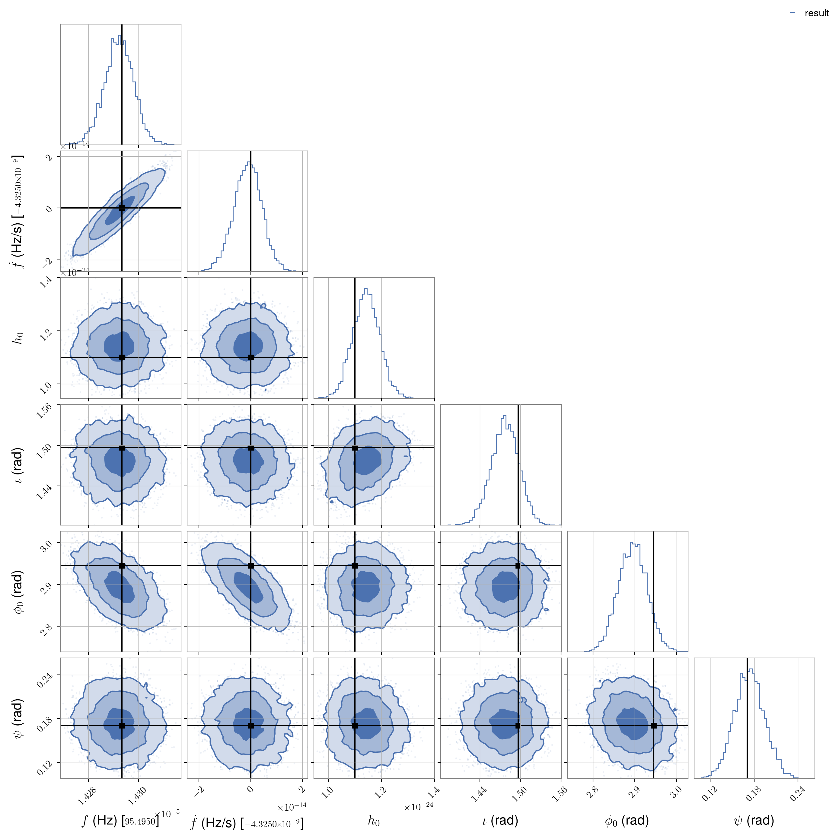
which shows that the frequency and frequency derivatives are found at the correct values well within the prior ranges.

Using ROQ with a search pipeline

The ROQ likelihood can be used within a search pipeline, i.e., when running cwinpy_knope_pipeline or cwinpy_pe_pipeline. This requires individual prior files to be specified for each source being searched for. Here, we will perform a search for three pulsars in LIGO O1 data:

• the hardware injections, PULSAR01 and PULSAR05, for which we will “accidentally” heterodyne using a slightly offset sky locations and then perform parameter estimation over a small sky patch including the true location;

• the pulsar PSR J1932+17, which was an outlier in the O1 analysis, for which we will search over a small frequency and frequency derivative range based on expanding the uncertainty given by the electromagnetic timing solution by a factor of 5.

For the PULSAR01 hardware injection, we will use a .par file containing

PSRJ    JPULSAR01
F0	424.5416481
F1	-1.50e-10
# ORIGINAL RIGHT ASCENSION
#RA	02:29:34.5244056970
RA      02:29:34.5381566841
# ORIGINAL DECLINATION
#DEC	-29:27:08.8572763812
DEC     -29:27:09.0635411874
PEPOCH	52944.0007428703684126958
UNITS   TDB
EPHEM   DE405
H0      2.19401964075e-24
IOTA    1.08849139457
PSI     0.35603553
PHI0    0.64

where the right ascension and declination have been shifted by 0.001 mrad (0.0138 seconds) and -0.001 mrad (-0.2063 arcsec), respectively, compared to their actual values. We will use a prior file that searches over right ascension and declination over a uniform patch spanning ±0.002 mrad in each coordinate (around the true values):

h0 = Uniform(minimum=0.0, maximum=1.0e-22, name='h0', latex_label='$h_0$')
phi0 = Uniform(minimum=0.0, maximum=3.141592653589793, name='phi0', latex_label='$\phi_0$', unit='rad')
iota = Sine(minimum=0.0, maximum=3.141592653589793, name='iota', latex_label='$\iota$', unit='rad')
psi = Uniform(minimum=0.0, maximum=1.5707963267948966, name='psi', latex_label='$\psi$', unit='rad')
ra = Uniform(minimum=0.652643832, maximum=0.652647832, name='ra', latex_label='$\alpha$', unit='rad')
dec = Uniform(minimum=-0.514044406, maximum=-0.514040406, name='dec', latex_label='$\delta$', unit='rad')

For the PULSAR05 hardware injection, we will use a .par file containing

PSRJ    JPULSAR05
F0	26.40416218
F1	-2.015e-18
# original RA
#RA	20:10:30.3939266193
RA 20:10:30.6689463610
# original DEC
#DEC	-83:50:20.9035791210
DEC -83:50:27.0915233084
PEPOCH	52944.0007428703684126958
UNITS   TDB
EPHEM   DE405
H0      1.46427693185e-24
IOTA    1.08945639689
# PSI = PSI_INJ + PI/2 = -0.363953188 + PI/2
PSI     1.206843138794896
# PHI0 = MOD((PHI_GW/2) + PI/2, PI) = MOD((2.23/2) + PI/2, PI)
PHI0    2.6857963267948968

where the right ascension and declination have been shifted by 0.02 mrad (0.275 seconds) and -0.03 mrad (-6.188 arcsec), respectively, compared to their actual values. These shifts are much larger than for PULSAR01 due to it being at a much lower frequency for which the sky resolution is poorer. We will use a prior file that searches over right ascension and declination over a uniform patch spanning ±0.05 mrad in each coordinate (around the true values):

h0 = Uniform(minimum=0.0, maximum=1.0e-22, name='h0', latex_label='$h_0$')
phi0 = Uniform(minimum=0.0, maximum=3.141592653589793, name='phi0', latex_label='$\phi_0$', unit='rad')
iota = Sine(minimum=0.0, maximum=3.141592653589793, name='iota', latex_label='$\iota$', unit='rad')
psi = Uniform(minimum=0.0, maximum=1.5707963267948966, name='psi', latex_label='$\psi$', unit='rad')
ra = Uniform(minimum=5.2817812959999975, maximum=5.281881295999997, name='ra', latex_label='$\alpha$', unit='rad')
dec = Uniform(minimum=-1.4633190329999997, maximum=-1.4632190329999994, name='dec', latex_label='$\delta$', unit='rad')

For PSR J1932+17, the .par file we will use (as can be found here) contains:

PSRJ	       J1932+17
RAJ            19:32:07.1674282          1  0.01023320381669795939   
DECJ           +17:56:18.70142           1  0.25231198765634132427   
F0             23.905550847651064273     1  0.00000000082758861857   
F1             -1.4458267504087269662e-15    6.7521640918638115878e-16
PEPOCH         56803.000211785492581       
POSEPOCH       56803.000211785492581
BINARY         ELL1
PB             41.507985998762112295     1  0.00000898573888192338   
A1             68.859148021929869263     1  0.00030720578073581612   
TASC           56765.946209275262305     1  0.00011436348933596476   
EPS1           -0.0001969460108668249454 1  0.00000737922338307618   
EPS2           0.00014522453787412931602 1  0.00000762676141481106   
UNITS          TCB
EPHEM          DE405

and the prior file is:

h0 = Uniform(minimum=0.0, maximum=1.0e-21, name='h0', latex_label='$h_0$')
phi0 = Uniform(minimum=0.0, maximum=3.141592653589793, name='phi0', latex_label='$\phi_0$', unit='rad')
iota = Sine(minimum=0.0, maximum=3.141592653589793, name='iota', latex_label='$\iota$', unit='rad')
psi = Uniform(minimum=0.0, maximum=1.5707963267948966, name='psi', latex_label='$\psi$', unit='rad')
f0 = Uniform(minimum=23.905550843513122, maximum=23.905550851789005, name='f0', latex_label='$f_0$', unit='Hz')
f1 = Uniform(minimum=-4.821908796340633e-15, maximum=1.930255295523179e-15, name='f1', latex_label='$\dot{f}$', unit='Hz/s')

The configuration file used is:

[run]
basedir = /home/matthew.pitkin/ROQ

[knope_job]
accounting_group = aluk.dev.o1.cw.targeted.bayesian
accounting_group_user = matthew.pitkin

[heterodyne]
detectors = 'H1'
starttimes = 1126051217
endtimes = 1137254417
frametypes = {'H1': 'H1_LOSC_16_V1'}
host = datafind.gwosc.org
channels = {'H1': 'H1:GWOSC-16KHZ_R1_STRAIN'}
includeflags = {'H1': 'H1_CBC_CAT1'}
excludeflags = {'H1': 'H1_NO_CW_HW_INJ'}
outputdir = {'H1': '/home/matthew.pitkin/ROQ/H1'}

[merge]
remove = True

[pe]
priors = {'JPULSAR01': '/home/matthew.pitkin/ROQ/PULSAR01_prior.txt', 'JPULSAR05': '/home/matthew.pitkin/ROQ/PULSAR05_prior.txt', 'J1932+17': '/home/matthew.pitkin/ROQ/ROQ_J1932+17_prior.txt'}
roq = True
sampler_kwargs = {'sample': 'rwalk'}
data_kwargs = {'bbminlength': 14400}

[pe_dag]
submitdag = True

[pe_job]
request_memory = 64GB

[ephemerides]
pulsarfiles = {'JPULSAR01': '/home/matthew.pitkin/ROQ/PULSAR01_offset.par', 'JPULSAR05': '/home/matthew.pitkin/ROQ/PULSAR05_offset.par', 'J1932+17': '/home/matthew.pitkin/ROQ/J1932+17.par'}

which is run with:

$ cwinpy_knope_pipeline roq_pipeline_example.ini

Attention

Note that in this configuration file, in the [pe] section, we have:

data_kwargs = {'bbminlength': 14400}

This defines the minimum “chunk length” into which the heterodyned data can split by the bayesian_blocks() method. The ROQ method will produce a reduced order quadrature for each data “chunk”, so setting this to 14,400 seconds (10 days) reduces the number of ROQs that are required to be calculated. However, this also means that the amount of memory required to run this needs to be increased, hence the lines:

[pe_job]
request_memory = 64GB

in the file.

It is also important to note that the sampling method used in

sampler_kwargs = {'sample': 'rwalk'}

is set to rwalk. While this is the default sampling method that CWInPy will use for the dynesty sampler, it is explicitly set here to note that for sampling over sky location this method (or similar) is required as opposed to the rslice method that was default for CWInPy versions between v0.8.0 and v0.10.0. It was found that rslice performed very poorly when sampling over sky position, most likely (although speculatively) due to the sky location being very tightly localised within the prior volume and slices very rarely intersecting with it.

Once complete, the posteriors for the J1932+17 analysis can be plotted with:

from cwinpy.plot import Plot
plot = Plot("cwinpy_pe_H1_J1932+17_result.hdf5")
plot.plot(bins=25)
plot.savefig("cwinpy_pe_J1932+17.png", dpi=200)

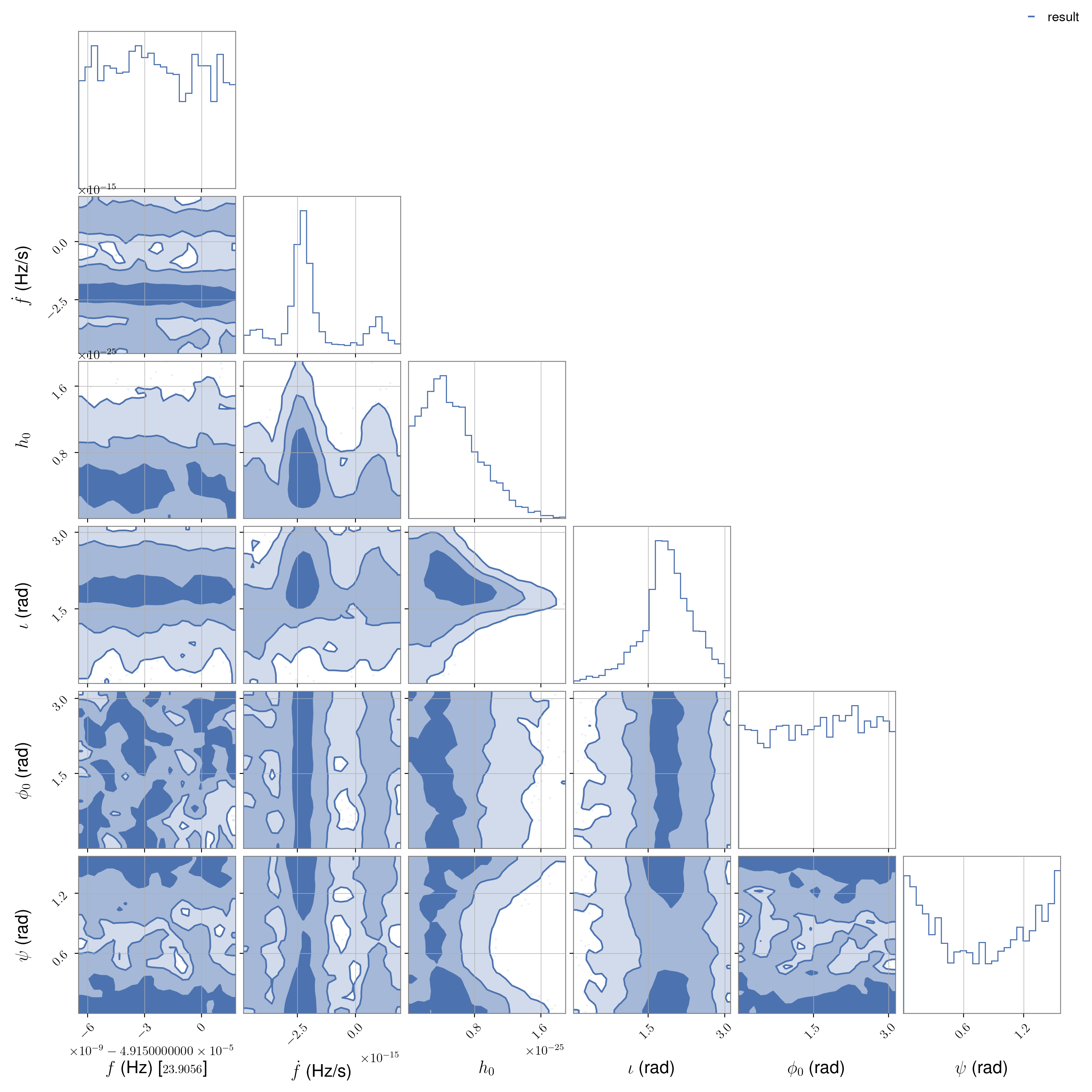
We can see that the posterior has a strong peak in the frequency derivative, which is primarily responsible for \(h_0\) peaking away from zero, although the posterior over frequency is rather unconstrained.

The posteriors for the PULSAR05 analysis can be plotted, along with the true injected values, using (where the sky position axes ranges have been expanded to show the full prior range and the offset sky location at which the heterodyne was performed is also shown in orange):

from cwinpy import HeterodynedData
from cwinpy.info import HW_INJ
from cwinpy.plot import Plot
plot = Plot(
   "cwinpy_pe_H1_JPULSAR05_result.hdf5",
   pulsar=HW_INJ["O1"]["hw_inj_files"][5]
)

# read in heterodyned data to extract heteroydne parameters
het = HeterodynedData.read("../../H1/heterodyne_JPULSAR05_H1_2_1129136736-1137253524.hdf5")

# plot showing full prior range over RA/DEC and original heterodyne position
fig = plot.plot()
ax = fig.axes

for axs in ax[::6]:
    axs.set_xlim(
        [
            plot.pulsar["DEC"] - plot.parameter_offsets["dec"] - 0.05e-3,
            plot.pulsar["DEC"] - plot.parameter_offsets["dec"] + 0.05e-3
        ]
    )
    axs.axvline(het.par["DEC"] - plot.parameter_offsets["dec"], color="tab:orange")

for axs in ax[-6:-1]:
    axs.set_ylim(
        [
            plot.pulsar["RA"] - plot.parameter_offsets["ra"] - 0.05e-3,
            plot.pulsar["RA"] - plot.parameter_offsets["ra"] + 0.05e-3
        ]
    )
    axs.axhline(het.par["RA"] - plot.parameter_offsets["ra"], color="tab:orange")

ax[-1].set_xlim(
    [
        plot.pulsar["RA"] - plot.parameter_offsets["ra"] - 0.05e-3,
        plot.pulsar["RA"] - plot.parameter_offsets["ra"] + 0.05e-3
    ]
)
ax[-1].axvline(het.par["RA"]- plot.parameter_offsets["ra"], color="tab:orange")
plot.savefig("cwinpy_pe_JPULSAR05.png", dpi=200)

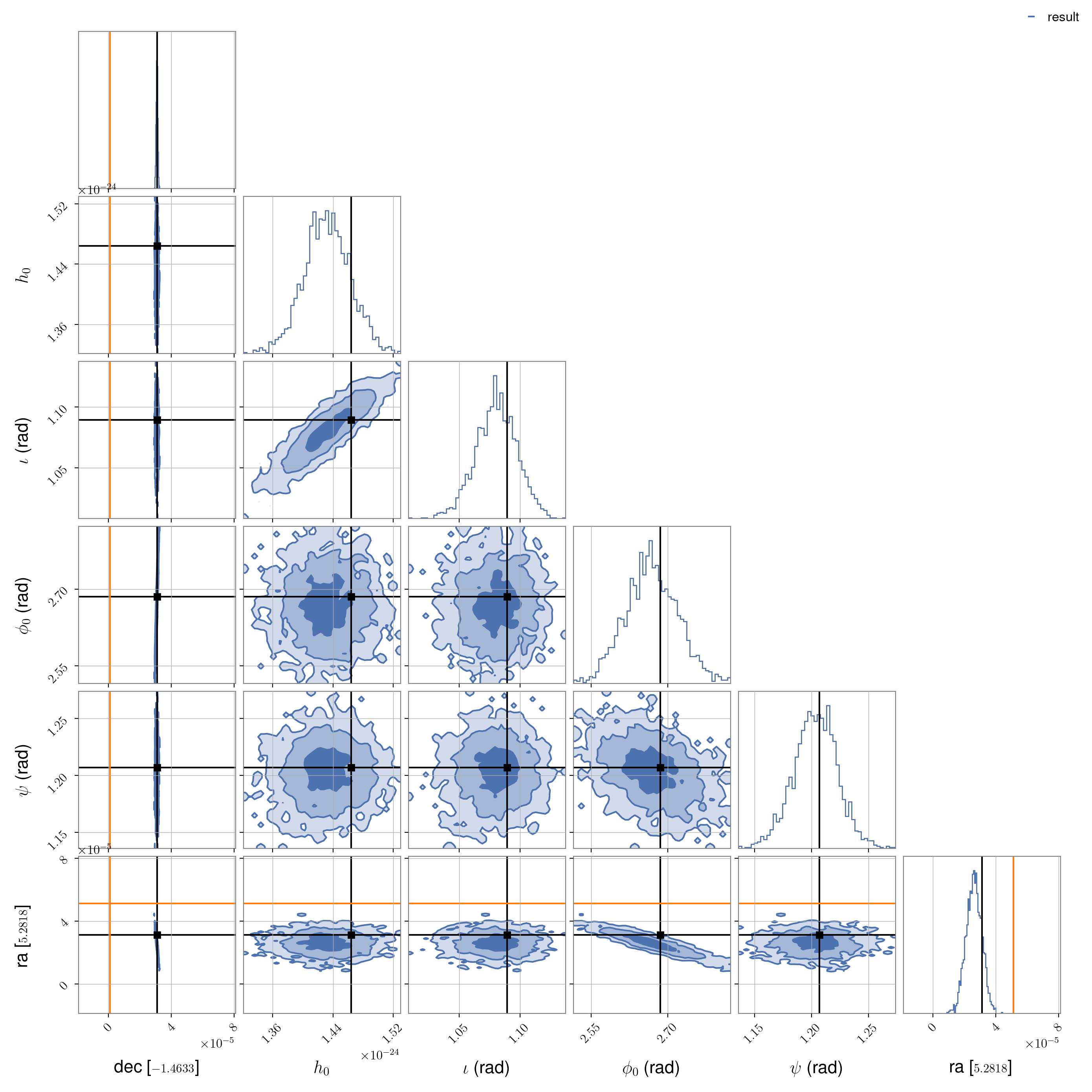
We see here that, despite the heterodyne offset in sky location, the true value has still been well recovered and the other source parameter are also recovered well (see `Injection parameter comparison`_ for comparison).

The posteriors for the PULSAR01 analysis can be plotted, along with the true injected values, using (where the sky position axes ranges have been expanded to show the full prior range and the offset sky location at which the heterodyne was performed is also shown in orange):

from cwinpy import HeterodynedData
from cwinpy.info import HW_INJ
from cwinpy.plot import Plot
plot = Plot(
   "cwinpy_pe_H1_JPULSAR01_result.hdf5",
   pulsar=HW_INJ["O1"]["hw_inj_files"][1]
)

# read in heterodyned data to extract heteroydne parameters
het = HeterodynedData.read("../../H1/heterodyne_JPULSAR01_H1_2_1129136736-1137253524.hdf5")

# plot showing full prior range over RA/DEC and original heterodyne position
fig = plot.plot()
ax = fig.axes

for axs in ax[::6]:
    axs.set_xlim(
        [
            plot.pulsar["DEC"] - plot.parameter_offsets["dec"] - 0.002e-3,
            plot.pulsar["DEC"] - plot.parameter_offsets["dec"] + 0.002e-3
        ]
    )
    axs.axvline(het.par["DEC"] - plot.parameter_offsets["dec"], color="tab:orange")

for axs in ax[-6:-1]:
    axs.set_ylim(
        [
            plot.pulsar["RA"] - plot.parameter_offsets["ra"] - 0.002e-3,
            plot.pulsar["RA"] - plot.parameter_offsets["ra"] + 0.002e-3
        ]
    )
    axs.axhline(het.par["RA"] - plot.parameter_offsets["ra"], color="tab:orange")

ax[-1].set_xlim(
    [
        plot.pulsar["RA"] - plot.parameter_offsets["ra"] - 0.002e-3,
        plot.pulsar["RA"] - plot.parameter_offsets["ra"] + 0.002e-3
    ]
)
ax[-1].axvline(het.par["RA"]- plot.parameter_offsets["ra"], color="tab:orange")
plot.savefig("cwinpy_pe_JPULSAR01.png", dpi=200)

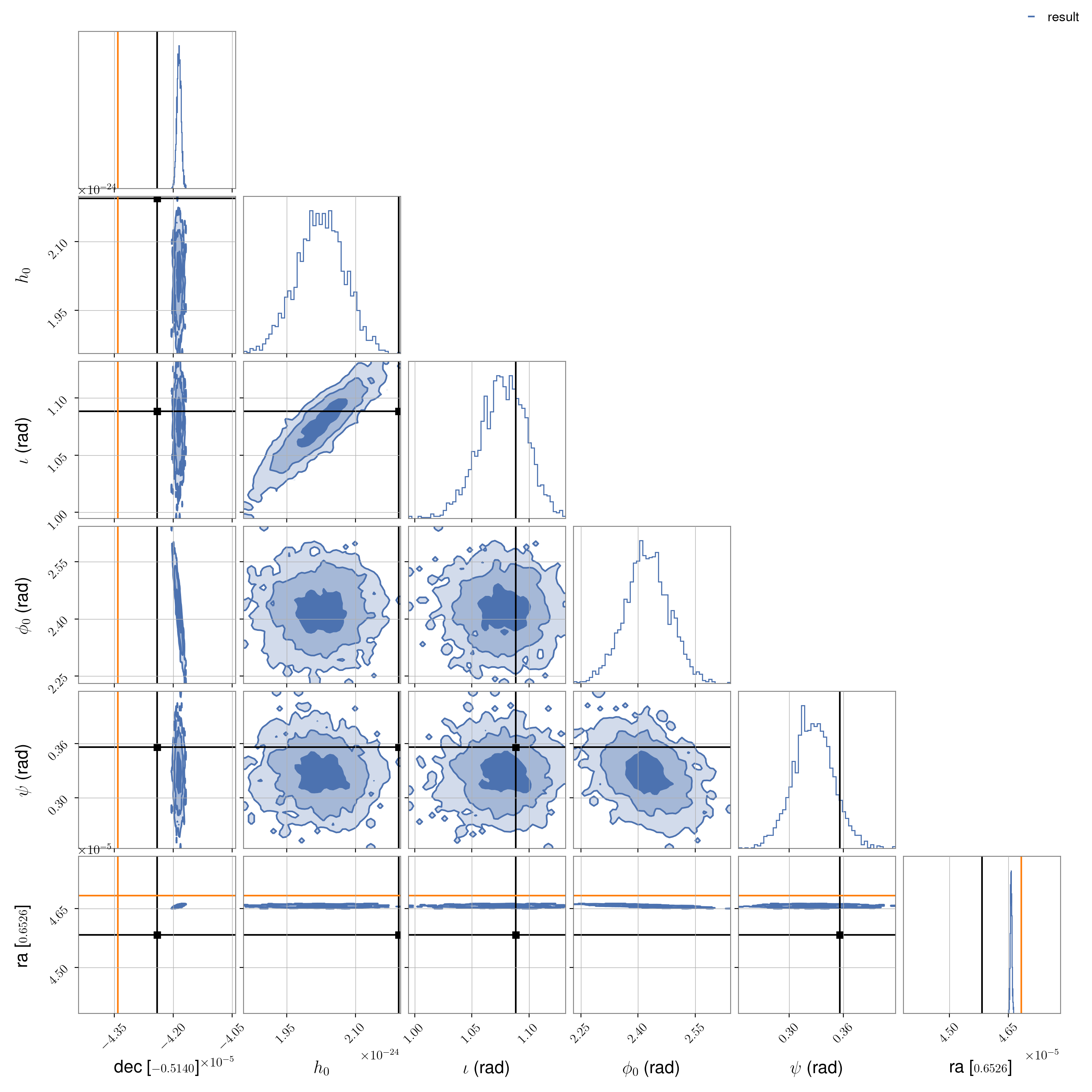
In this case, we see that the recovered sky location does not match the true location or the offset location at which the heterodyned was performed! However, the other parameters are recovered as expected, or at least consistently with those recovered in `Injection parameter comparison`_, suggesting that the recovered location is a “good” one. A reason behind this discrepancy may lie in the generation of the hardware injections themselves. For the injections, the sky-location dependent time-delays are calculated from a look-up table generated every 800 seconds (see descriptions here). This has been seen in the past (LVK-only link) to cause small phase discrepancies, which may be being modelling in this analysis (for which the time-delays are calculated and interpolated between on 60 second intervals during the heterodyne and for every time point during the ROQ generation) as a sky location offset. This is seen for PULSAR01 rather than the PULSAR05 analysis above due to its higher frequency and its respectively finer sky resolution.

ROQ API

The API for the ROQ generation class is given below. In general, direct use of this class is not required and generation of ROQ for likelihoods will be performed via the TargetedPulsarLikelihood class and the generate_roq() method of the HeterodynedData class.

class GenerateROQ(data, x, priors, **kwargs)

Bases: object

Generate the Reduced Order Quadrature for the parameters in the prior.

Parameters:

• data (array_like) – The data set (real or complex) for which the ROQ will be produced.

• x (array_like) – The values at which the data is defined (e.g., a set of times).

• priors (PriorDict) – A PriorDict containing the parameters and prior distributions, which will be used to generate the model reduced basis set.

• ntraining (int) – The number of training example models to be generated from which to produce the reduced basis set. Defaults to 5000.

• sigma (array_like, float) – The noise standard deviation for the data, which is assumed to be stationary over the data. If not given, this will be assume to be 1.0 for all data points.

• store_training_data (bool) – If set to True the class will store the array of models used to generate the reduced basis. Note that if using this class multiple times, storing the data could become memory intensive. Defaults to False.

• greedy_tol (float) – The tolerance to use when generating the reduced basis. Defaults to 1e-12.

• model (func) – The model function used to generate the training examples. By default this assumes the cwinpy.signal.HeterodynedCWSimulator as the model (see Other Parameters below), but it can be an arbitrary Python function provided the function has an initial positional argument that takes in the x values, followed by keyword arguments for the other function parameters as defined in the priors.

Other Parameters:

• par (PulsarParameters) – A cwinpy.parfile.PulsarParameters or parameter file containing the parameters used for heterodyning the data.

• det (str) – The name of the detector for which the signal will be modelled.

• usetempo2 (bool) – Set to True if the signal model phase evolution should be calculated using Tempo2. Defaults to False.

generate_reduced_basis(training)

Generate the reduced basis for the training set.

generate_training_set()

Generate n model instances, using values drawn from the prior.

log_likelihood(**kwargs)

Calculate the log-likelihood using the reduced order basis.

Parameters:

likelihood (str) – When calculating the ROQ likelihood, set whether it is a Gaussian likelihood "gaussian" or Student’s t-likelihood "studentst". As with the cwinpy.pe.likelihood.TargetedPulsarLikelihood, the default is Student’s t.

ROQ References

[1]

H. Antil et al., Journal of Scientific Computing, 57, 604-637 (2013).

[2] (1,2)

P. Canizares, S. E. Field, J. R. Gair & M. Tiglio, PRD, 87, 124005 (2013).

[3]

M. Tiglio & A. Villanueva, LRR, 25, 2 (2022).

[4]

M. Pitkin, M. Isi, J. Veitch & G. Woan, arXiv:1705.08978v1, 2017.