Pulsar simulations#
You can use CWInPy to generate a simulated population of neutron star sources that can be used for subsequent parameter estimation and hierarchical analyses. Currently, the simulation code assumes a source signal model from a rigid triaxial rotator emitting from the \(l=m=2\) quadrupole mode. It is also assumes that the simulated population are known pulsars and therefore the data has been heterodyned using a known phase evolution.
The simulation can either: generate a selection of entirely fake pulsars, with distributions for amplitude (defined through either the gravitational-wave strain amplitude \(h_0\), the mass quadrupole \(Q_{22}\), or the ellipticity), source location (right ascension, declination and distance) and pulsar orientation parameters supplied by the user (or set to defaults for everything other than \(Q_{22}\)); or, use supplied pulsars parameters and heterodyned data into which to inject signals drawn from a population of \(Q_{22}\).
The simulations are generated using the PEPulsarSimulationDAG
class which is described at the bottom of the page. Note that the simulation code described here
does not actually create the simulated gravitational-wave detector data. This is done in the
individual cwinpy_pe jobs generated by the script.
Simulation using fake data#
As a first example we will create a simulation that generates a population of 1000 pulsars with their \(Q_{22}\) values drawn from an exponential distribution with a mean of 1033 kg m2, and sets up parameter estimation jobs for each. This population will be drawn from the default distribution on the pulsar location (uniform over the sky and uniform within a distance range between 0.1 and 10 kpc) and the default distribution on the pulsar orientation (uniform on the hemisphere in inclination and polarisation angle and uniform in initial phase). We will set a prior for the parameter estimation that has a uniform distribution in \(Q_{22}\) between 0 and 1040 kg m2.
from cwinpy.pe.simulation import PEPulsarSimulationDAG
from bilby.core.prior import PriorDict, Uniform, Exponential, Sine
import numpy as np

# set the Q22 distribution
mean = 1e33
ampdist = Exponential(name="q22", mu=mean)

# set the prior distribution for use in parameter estimation
prior = PriorDict({
    "q22": Uniform(0.0, 1e40, name="q22"),
    "iota": Sine(name="iota"),
    "phi0": Uniform(0.0, np.pi, name="phi0"),
    "psi": Uniform(0.0, np.pi / 2, name="psi"),
})

# set the detectors to use (and generate fake data for)
detectors = ["H1", "L1"]

# generate the population
run = PEPulsarSimulationDAG(ampdist=ampdist, prior=prior, npulsars=1000, detector=detectors)
As no basedir argument was supplied this will produce the following directories and files in
your current working directory:
$ ls -p
configs/  log/  priors/  pulsars/  results/ submit/
The pulsars directory will contain the 1000 pulsar parameter files with names based on their
generated right ascension and declination (clashing positions will have alphabetical identifiers
appended). The priors directory will contain 1000 prior files named after each pulsar. The
configs directory will contain the 1000 cwinpy_pe configuration files. The results directory will be where a directory for each pulsar’s results outputs
will be placed. The submit directory will contain the files required for running the HTCondor
DAG. There will be a Condor submit
file for each pulsar, which by default will be labelled cwinpy_pe_PSRNAME.submit`, where
``PSRNAME will be the pulsar name (note that names based on a positive declination will have +
replaced with plus to make them allowable Condor job names). There will also be a
dag_cwinpy_pe.submit file containing the HTCondor DAG file. The log directory will contain
the log files for each of the jobs.
Note
For each pulsar you can run multiple parallel independent runs that will be merged by using the
n_parallel option of PEPulsarSimulationDAG. This will create
configuration files and submit files for each of the parallel runs. In the results directory for
each pulsar a par{NUM} directory will be created for each parallel run, where {NUM} runs
from 0 to one less than the number of parallel runs. The results of the parallel runs will be
merged as part of the DAG, so the submit directory will also contain submit files for the merge
jobs.
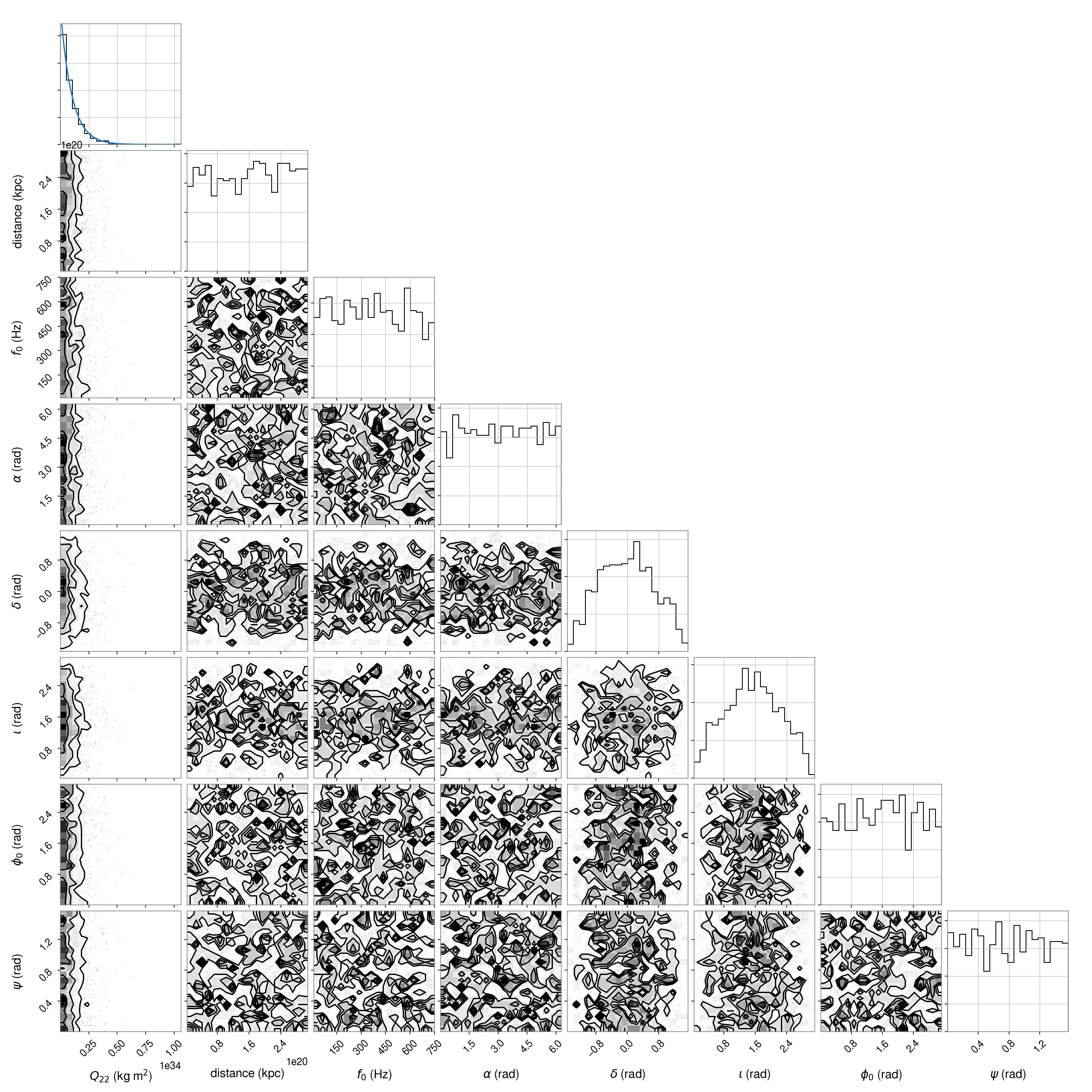
We can take a look at the distribution of parameters that gets produced with:
import corner
import glob
import numpy as np
from cwinpy import PulsarParameters

params = np.zeros((1000, 8))
for i, parfile in enumerate(glob.glob("pulsars/*.par")):
    psr = PulsarParameters(parfile)
    params[i, :] = [psr["Q22"], psr["DIST"], psr["F0"], psr["RAJ"], psr["DECJ"], psr["IOTA"], psr["PHI0"], psr["PSI"]]

# make a corner plot of the distributions
labels = [r"$Q_{22}$ (kg m$^2$)", "distance (kpc)", r"$f_0$ (Hz)", r"$\alpha$ (rad)", r"$\delta$ (rad)", r"$\iota$ (rad)", r"$\phi_0$ (rad)", r"$\psi$ (rad)"]
fig = corner.corner(params, labels=labels, hist_kwargs={"density": True})

# overplot the Q22 distribution
ax = fig.get_axes()
lims = ax.get_xlim()
q22s = np.linspace(lims[0], lims[1], 100)
ax[0].plot(q22s, q22dist.prob(q22s))
If you are on a machine, or computer cluster, with HTCondor installed these parameter estimation jobs can be run using
$ condor_submit_dag cwinpy_pe_pipeline_DATETAG_01.submit
where DATETAG is a date string in the DAG file name based on the date you created it on.
You can perform an analysis using simulated data, but with real (or pre-defined) pulsar parameter
files. If you have a set of pulsar parameters files then these can be passed to the
PEPulsarSimulationDAG class by giving a directory containing all the
files, or a dictionary of file paths keyed to the pulsar names. This takes the place of supplying a
number of pulsars to be simulated. For example, if we had parameter files in the directory
my_pulsars this could be used with:
pardir = "my_pulsars"
run = PEPulsarSimulationDAG(ampdist, prior=prior, parfiles=pardir, detector=detectors)
Note that you should not call the parameter file directory pulsars if it is in the same base
directory that you are generating the simulation in. That directory is reserved for pulsar parameter
files that contain the simulated population signal parameters for adding into the data.
Different distributions#
You do not have to use the default distributions on the pulsar positions or orientation parameters. If you had a model for a location distribution (and it can be put in the form of a bilby prior) in equatorial (right ascension and declination) or Galactic (galactic longitude and latitude) coordinates and distance, or cartesian Galactocentric coordinates (in kpc), then these can be used.
If using the equatorial system the prior dictionary must be keyed with "ra", "dec" and
"dist" with angles in radians and distance in kpc. If using the Galactic coordinate system the
prior dictionary must be keyed with "l", "b" and "dist", again with angles in radians
and distance in kpc. For the Galactocentric system the prior dictionary must be keyed with "x",
"y" and "z" in kpc.
For example, suppose we modelled the Galaxy as a thin Gaussian disk with a scale (standard deviation of the Gaussian) of 9 kpc in the x-y plane, and 0.15 kpc in the z-direction, we could use this for our pulsar population with:
from bilby.core.prior import PriorDict, Gaussian
posdist = PriorDict({
"x": Gaussian(0.0, 9.0, name="x"),
"y": Gaussian(0.0, 9.0, name="y"),
"z": Gaussian(0.0, 0.15, name="z"),
})
run = PEPulsarSimulationDAG(
ampdist, npulsars=1000, detector=detectors, posdist=posdist,
)
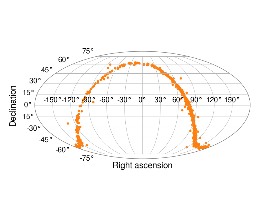
# let's plot the sky distribution in RA and dec
from matplotlib import pyplot as pl
import glob
import numpy as np
from cwinpy import PulsarParameters
params = np.zeros((1000, 2))
for i, parfile in enumerate(glob.glob("pulsars/*.par")):
psr = PulsarParameters(parfile)
params[i, :] = [-psr["RAJ"] if psr["RAJ"] < np.pi else -(psr["RAJ"] - 2 * np.pi), psr["DECJ"]]
fig, ax = pl.subplots(1, 1, subplot_kw={"projection": "mollweide"})
ax.scatter(params[:,0], params[:,1], s=8)
ax.set_xlabel("Right ascension")
ax.set_ylabel("Declination")
fig.savefig("mollweide.png", dpi=150, tight_layout=True)
If we wanted to fix a parameter like right ascension then we could use a Delta function prior in that parameter, e.g.:
from bilby.core.prior import PriorDict, DeltaFunction, Uniform, Cosine
posdist = PriorDict({
    "ra": DeltaFunction(1.3, name="ra"),  # fix RA at 1.3 radians
    "dec": Cosine(name="dec"),
    "dist": Uniform(0.1, 10.0, name="dist"),
})
The source orientation parameter distribution can also be set to something other than the default. For example, to set the sources to all be linearly polarised you could use:
from bilby.core.prior import PriorDict, DeltaFunction
oridist = PriorDict({
    "iota": DeltaFunction(np.pi / 2., name="iota"),
})
run = PEPulsarSimulationDAG(
    ampdist, npulsars=100, detector=detectors, oridist=oridist,
)
In this case, as the other orientation parameters are not supplied they will automatically get set to their default distributions.
Simulating a realistic distribution#
Rather than guessing at a pulsar distribution we could try and use the true distribution of pulsars. To do this we can make use of the psrqpy package to get the currently known pulsars from the ATNF pulsar catalogue, and, for example, the astroML package [1] to fit the distribution using a Gaussian Mixture Model via extreme deconvolution [2] (other packages can be used for this).
from psrqpy import QueryATNF
from astroML.density_estimation import XDGMM
from matplotlib import pyplot as pl
import glob
import numpy as np
from cwinpy import PulsarParameters
from cwinpy.pe.simulation import PEPulsarSimulationDAG
from bilby.core.prior import PriorDict, Uniform, Exponential, Sine
# get the Galactic X, Y, Z coordinates for all pulsars (excluding Globular Clusters)
query = QueryATNF(params=["XX", "ZZ", "YY", "RAJD", "DECJD"], condition="~assoc(GC)")
# extract the position values and put them into an array
t = query.table
mask = ~t["XX"].data.mask # values that are not masked (e.g., NaNs)
positions = np.vstack(
(t["XX"].data.data[mask], t["YY"].data.data[mask], t["ZZ"].data.data[mask])
).T
# initialise the extreme deconvolution (try 20 components)
gmm = XDGMM(n_components=20, max_iter=500, tol=1e-2, verbose=True)
# set some errors on the positions (required for XDGMM), say 5% on all values
dx = positions[:,0] * 0.05
dy = positions[:,1] * 0.05
dz = positions[:,2] * 0.05
poserr = np.zeros(positions.shape + positions.shape[-1:])
diag = np.arange(positions.shape[-1])
poserr[:, diag, diag] = np.vstack([dx ** 2, dy ** 2, dz ** 2]).T
# fit the positions (this may take some time!)
gmm.fit(positions, Xerr=poserr)
# set a Multivariate Gaussian distribution
names = ["x", "y", "z"]
mvg = bilby.core.prior.MultivariateGaussianDist(
names,
nmodes=20,
mus=gmm.mu.tolist(),
covs=gmm.V.tolist(),
weights=gmm.alpha.tolist(),
)
# set the position distribution as a bilby Prior
posdist = PriorDict()
for name in names:
posdist[name] = bilby.core.prior.MultivariateGaussian(mvg, name)
# create a simulated population of pulsars
detectors = "H1"
mean = 1e33
ampdist = Exponential(name="q22", mu=mean)
run = PEPulsarSimulationDAG(
ampdist, npulsars=1000, detector=detectors, posdist=posdist,
)
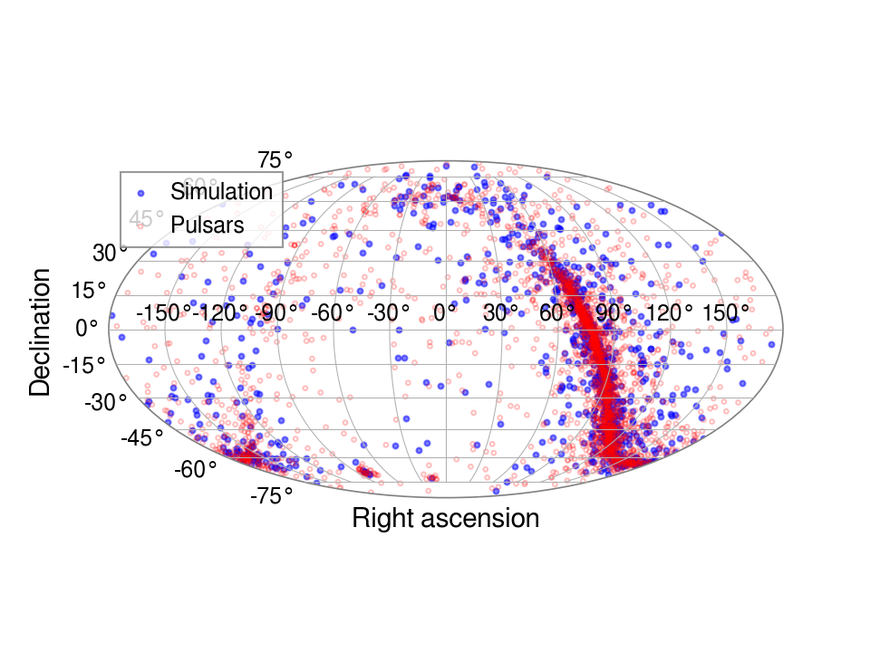
# plot the distribution (c)
params = np.zeros((1000, 2))
for i, parfile in enumerate(glob.glob("pulsars/*.par")):
psr = PulsarParameters(parfile)
params[i, :] = [-psr["RAJ"] if psr["RAJ"] < np.pi else -(psr["RAJ"] - 2 * np.pi), psr["DECJ"]]
pparams = np.zeros((len(t), 2))
for i, rasdecs in enumerate(zip(np.deg2rad(t["RAJD"]), np.deg2rad(t["DECJD"]))):
pparams[i, :] = [-rasdecs[0] if rasdecs[0] < np.pi else -(rasdecs[0] - 2 * np.pi), rasdecs[1]]
fig, ax = pl.subplots(1, 1, subplot_kw={"projection": "mollweide"})
ax.scatter(params[:,0], params[:,1], s=8, color="b", alpha=0.5, label="Simulation")
ax.scatter(pparams[:,0], pparams[:,1], s=5, color="none", edgecolor="r", alpha=0.25, label="Pulsars")
ax.set_xlabel("Right ascension")
ax.set_ylabel("Declination")
ax.legend()
fig.savefig("distribution.png", dpi=150, tight_layout=True)
A similar thing could be done to generate the distribution of pulsar frequencies.
Distance uncertainty#
You may want to run parameter estimation on a simulation for which you include a prior on the
distance for each pulsar. One way to do this when using a selection of pregenerated or real pulsars
is to pass the prior argument a dictionary of prior files or bilby PriorDict’s, keyed to
each pulsar, which contain a "dist" value with the particular distance prior required. This can
also be achieved by instead passing a dictionary of priors, or dictionary of distance standard
deviations (in kpc), keyed to the pulsar names, to the distance_err argument, e.g.,:
from bilby.core.prior import Gaussian, Uniform, Sine, PriorDict, Exponential

# assume we have two pulsars (J0000+0000 and J0100+0100) with parameter
# files in the directory "pardir" for which we will set Gaussian priors
# with standard deviations of 0.3 and 0.2 kpc, respectively.
dist_err = {"J0000+0000": 0.3, "J0100+0100": 0.2}
prior = PriorDict({
    "q22": Uniform(0.0, 1e40, name="q22"),
    "iota": Sine(name="iota"),
    "phi0": Uniform(0.0, np.pi, name="phi0"),
    "psi": Uniform(0.0, np.pi / 2, name="psi"),
})
ampdist = Exponential(name="q22", mu=1e33)
run = PEPulsarSimulationDAG(
    ampdist=ampdist, parfiles="pardir", prior=prior, distance_err=dist_err, detector="H1"
)
Note
In the latter case it will generate a Gaussian prior on the distance and assumes that the pulsar distance is given as this is used as the mean of the distribution.
If generating a population of pulsars, you can use the distance_err argument to set a Gaussian
distance prior for all pulsars. If you pass a number it will be taken as the fractional distance
uncertainty and used to set the standard deviation of a Gaussian distribution (truncated at zero),
with a mean based on the distance that is drawn for that source. At the moment this can only be a
single fractional error on the distance used for all pulsars.
Simulation using real data#
Rather than the simulation running on simulated data and simulated pulsars the code can be used to add signals to a set of real data and use pre-defined or real pulsar parameter files.
We will assume the following example directory tree for which there are heterodyned data files for a selection of pulsars and for two detectors (H1 and L1):
root
 ├── data          # directory to contain the heterodyned data for all pulsars
 |    ├── H1       # directory to contain the H1 data for all pulsars
 |    |    ├── fine-H1-pulsar1.txt  # heterodyned data for pulsar1 (file must contain the pulsar name)
 |    |    ├── fine-H1-pulsar2.txt  # heterodyned data for pulsar2
 |    |    └── ...
 |    └── L1       # directory to contain the L1 data for all pulsars
 |         ├── fine-L1-pulsar1.txt  # heterodyned data for pulsar1 (file must contain the pulsar name)
 |         ├── fine-L1-pulsar2.txt  # heterodyned data for pulsar2
 |         └── ...
 └── pulsars       # directory containing pulsar parameter files used for heterodyning
We could run a simulation that adds signals to these with mass quadrupoles drawn from an exponential distribution using:
from bilby.core.prior import PriorDict, Uniform, Exponential, Sine
from cwinpy.pe.simulation import PEPulsarSimulationDAG
import numpy as np

prior = PriorDict({
    "q22": Uniform(0.0, 1e36, name="q22"),
    "iota": Sine(name="iota"),
    "phi0": Uniform(0.0, np.pi, name="phi0"),
    "psi": Uniform(0.0, np.pi / 2, name="psi"),
})

detectors = ["H1", "L1"]
mean = 1e32  # the mean of the exponential distribution
ampdist = Exponential(name="q22", mu=mean)

# a dictionary of data file directories keyed to the detector
datafiles = {"L1": "/root/data/L1", "H1": "/root/data/H1"}

# the directory containing the pulsar parameter files
parfiles = "/root/pulsars"

run = PEPulsarSimulationDAG(
    ampdist=ampdist,
    prior=prior,
    datafiles=datafiles,
    parfiles=parfiles,
)
Note
The original data files are not changed by the simulation, so they will not contain the simulated signals.
By default, if the pulsar parameter files contain gravitational wave parameters (the amplitude or
mass quadrupole, and orientation parameters) or the distance, then these will be overwritten (in new
versions of the files) by any parameters generated in the simulation. If you want to keep those
parameters then the overwrite_parameters argument can be set to False.
Simulation class API#
The API for the PEPulsarSimulationDAG class is described below: