Hierarchical analyses

For a pulsar to emit gravitational waves it must have a time varying mass quadrupole. The strength of the observed gravitational-wave signal is proportional to the star’s mass quadrupole moment \(Q_{22}\), which is related to the star’s fiducial ellipticity [1]. Using gravitational-wave observations, an individual pulsar’s \(Q_{22}\) can be estimated, resulting in a posterior probability distribution marginalised over other parameters of the gravitational-wave signal (this can include the pulsar’s distance if a prior on the distance is known). However, a priori, the underlying distribution of \(Q_{22}\) (or equivalently ellipticity) for the pulsar population is unknown. This is where hierarchical Bayesian analysis comes in. If you chose a parameterisable distribution as a prior for the underlying \(Q_{22}\) distribution, then posteriors from multiple gravitational-wave pulsar observations can be combined, included those where no signal is detected, to estimate the parameters (known as hyperparameters) of that distribution [2]. For observations of \(N\) pulsars, the combined data from which is represented by \(\mathbf{D}\), and assuming a prior distribution for \(Q_{22}\) defined by a set of hyperparameters \(\vec{\theta}\), \(p(Q_{22}|\vec{\theta},I)\), then the posterior for \(\vec{\theta}\) is given by:

\[p(\vec{\theta}|\mathbf{D}, I) = \left(\prod_{i=1}^N \int^{{Q_{22}}_i} p(\mathbf{d}_i|{Q_{22}}_i,I) p({Q_{22}}_i|\vec{\theta},I) {\textrm d}{Q_{22}}_i\right) p(\vec{\theta}|I),\]

where \(p(\mathbf{d}_i|{Q_{22}}_i,I)\) is the marginalised likelihood distribution on \(Q_{22}\) for an individual pulsar given it’s observations \(\mathbf{d}_i\), and \(p(\vec{\theta}|I)\) is the prior on the hyperparameters.

The hierarchical module in CWInPy allows the outputs of pulsar parameter estimation for multiple sources to be combined to estimate the hyperparameters of several different potential \(Q_{22}\) (or ellipticity) distributions. To do this it is required that the parameter estimation has been performed using \(Q_{22}\) when defining the signal amplitude, rather than \(h_0\), and that the distance is either assumed to be precisely known, or the parameter estimation has included distance within the estimation via the use of a distance prior.

Evaluating the integral

Within the CWInPy implementation there are two ways provided of evaluating the integrals in the equation for \(p(\vec{\theta}|\mathbf{D}, I)\).

The first method is to evaluate the integrals numerically. A Gaussian kernel density estimate (KDE) of the posterior distribution \(p({Q_{22}}_i|\mathbf{d}_i,I)\) is generated for each pulsar, which is converted back into the required likelihood distribution via

\[p(\mathbf{d}_i|{Q_{22}}_i,I) = \frac{p({Q_{22}}_i|\mathbf{d}_i,I)}{p({Q_{22}}_i|I)} p(\mathbf{d}_i|I)\]

where \(p({Q_{22}}_i|I)\) is the prior on \(Q_{22}\) used during the parameter estimation and \(p(\mathbf{d}_i|I)\) is the marginal likelihood given the data for the i^th pulsar.

The second method uses the fact that the integrals are equivalent to calculating the expectation value of the prior distribution (see, e.g., [3]):

\[\mathrm{E}[p({Q_{22}}_i|\vec{\theta},I)] = \int^{{Q_{22}}_i} p(\mathbf{d}_i|{Q_{22}}_i,I) p({Q_{22}}_i|\vec{\theta},I) {\textrm d}{Q_{22}}_i \approx \frac{1}{M} \sum_{j=1}^M p({Q_{22}}_{i,j}|\vec{\theta},I),\]

where the term on the right hand side is calculating the mean of the \(Q_{22}\) distribution evaluated at the \(M\) samples from likelihood. In the case that the prior used for \(Q_{22}\) during the parameter estimation was not uniform then the MassQuadrupoleDistribution class will attempt to recreate likelihood samples by reweighting the posterior samples. In this case the scaling factor from the marginal likelihood is not included, however, Bayes factors for different distributions using the same data still can still be calculated.

Note

Both these methods should be equivalent, but as discussed in [2], for the particular case of estimating the pulsar mass quadrupole distribution, the “expectation value” method appears to suffer from numerical issues. This is particularly prominent for cases where to are no significantly detected signals for any pulsar, although it appears to have some effect even when strong signals are present (see the example below). It is not yet clear what the cause of the numerical issues is, but it appears to be related to the reasonably large dynamic range of possible hyperparameters (spanning several orders of magnitude) and the finite sampling of posteriors over that range.

It is therefore, for the moment, recommended to use the numerically evaluated integral based on KDEs of the posteriors.

Available distributions

The currently allowed distributions are:

• a mixture model of bounded Gaussian distributions: BoundedGaussianDistribution (where the “bounding” refers to the distributions being constrained to positive values as \(Q_{22}\) must be positive)

• an exponential distribution: ExponentialDistribution

• a power law distribution: PowerLawDistribution

• a delta function distribution: DeltaFunctionDistribution

• a non-parametric histogram-type distribution HistogramDistribution (see, e.g.,

The MassQuadrupoleDistribution can use any of the above distributions to define the distribution on the mass quadrupole to be inferred from a set of individual pulsar mass quadrupole posteriors.

When creating instances of these distributions via the create_distribution() function the following shorthand names can be used:

• "gaussian" for the BoundedGaussianDistribution

• "exponential" for the ExponentialDistribution

• "powerlaw" for the PowerLawDistribution

• "deltafunction" for the DeltaFunctionDistribution

• "histogram" for the HistogramDistribution

with the required hyperparameters as given by DISTRIBUTION_REQUIREMENTS. These names can also be used for the distribution argument of MassQuadrupoleDistribution.

Example

In this example we will use the simulation module to generate a set of pulsars with mass quadrupoles drawn from an exponential distribution and then show how the mean of that exponential distribution can be estimated.

The code below will generate a HTCondor DAG that will simulate 100 pulsars with \(Q_{22}\) values drawn from an exponential distribution with a mean of \(\mu = 10^{30}\, {\textrm{kg}}\,{\textrm m}^2\). The pulsars’ sky locations will be drawn uniformly over the sky and from the default uniform distance distribution. The orientations of the pulsars will also be drawn from the default uniform distributions, which are described in the PEPulsarSimulationDAG documentation. The simulation will only generate observations from a single gravitational-wave detector, the LIGO Hanford detector (“H1”), in this case.

The parameter estimation performed on each of these pulsars will use a uniform prior on \(Q_{22}\), a uniform prior over the orientation parameters (within the non-degenerate ranges), and will assume the distance to each is precisely know and equal to the simulated value.

from cwinpy.pe.simulation import PEPulsarSimulationDAG
from bilby.core.prior import PriorDict, Uniform, Exponential, Sine

# set the Q22 distribution
mean = 1e30
q22dist = Exponential(name="q22", mu=mean)

# set the prior for each pulsar
prior = PriorDict({
    "q22": Uniform(0.0, 1e38, name="q22"),
    "iota": Sine(name="iota"),
    "phi0": Uniform(0.0, np.pi, name="phi0"),
    "psi": Uniform(0.0, np.pi / 2, name="psi"),
})

# set the detector
detectors = ["H1"]

npulsars = 100  # number of pulsars to simulate

# generate and submit the simulation DAG
run = PEPulsarSimulationDAG(
    ampdist=ampdist,
    prior=prior,
    npulsars=npulsars,
    detector=detectors,
    basedir="/home/user/exponential",  # base directory for analysis output
    submit=True,  # automatically submit the HTCondor DAG
    numba=True,   # use numba for likelihood evaluation
    sampler_kwargs={'Nlive': 1000, 'sample': 'rwalk'},
)

Note

If running on LSC DataGrid computing resources the accountuser argument may be required to set the HTCondor accounting_group_user variable to your albert.einstein@ligo.org username, and accountgroup may be required to set the accounting_group variable to a valid accounting tag. You may also need to run ligo-proxy-init -p albert.einstein prior to submitting the HTCondor DAG that is generated.

Once the parameter estimation jobs have completed there should be a results directory within the directory specified by the basedir argument to PEPulsarSimulationDAG, which contains the results from each pulsar in the simulation. These can be combined to infer the hyperparameter of the \(Q_{22}\) distribution. Here we show how to do this using both methods of evaluating the marginalisation integrals described above, and estimating the posterior on the hyperparameters using both stochastic sampling (in this case using the nested sampling algorithm implemented in dynesty) and over a grid of points. The former methods is maybe over-the-top for this single dimensional example, but does have the advantage that the range and resolution of the required grid does not need to be known a priori.

Sampling the hyperparameters

To start with, the results for each pulsar need to be read in. This can be done using a bilby ResultList object using (assuming the base directory given above):

import glob
from bilby.core.result import ResultList

# get a list of result files
resultfiles = glob.glob("/home/user/exponential/results/J*/*.json")

# read in as list of bilby Result objects
data = ResultList(resultfiles)

Then a MassQuadrupoleDistribution needs to be set up and provided with the type of distribution for which the hyperparameters will be estimated, the priors on those hyperparameters, the method of evaluating the integrals, and any arguments required for the stochastic or grid-based sampling method. In this case the distribution is an exponential, and we will use a HalfNormal prior (a Gaussian distribution with a mode a zero, but excluding negative values) for the hyperparameter \(\mu\), with a scale parameter \(\sigma = 10^{34}\,{\textrm{kg}}\,{\textrm m}^2\) roughly based on the largest sustainable quadrupole deformations as described in [1].

The first example below uses the integral evaluation method that performs the integrals over \(Q_{22}\) numerically with the trapezium rule, which requires the "numerical" argument, and uses the default nested sampling routine to draw the samples from \(\mu\).

# set the distribution type
distribution = "exponential"

# set the hyperparameter prior distribution using a dictionary
sigma = 1e34
distkwargs = {"mu": HalfNormal(sigma, name="mu")}

# integration method
intmethod = "numerical"  # use the numerical trapezium rule integration over Q22

# set the sampler keyword arguments
sampler_kwargs = {
    "nlive": 500,
    "gzip": True,
    "outdir": "exponential_distribution",
    "label": intmethod,
    "check_point_plot": False,
}

# create the MassQuadrupoleDistribution object
mqd = MassQuadrupoleDistribution(
    data=data,
    distribution="exponential",
    distkwargs=distkwargs,
    sampler_kwargs=sampler_kwargs,
    integration_method=intmethod,
    nsamples=500,  # number of Q22 samples to store/use
)

# run the sampler
res = mqd.sample(sample="unif")

The res value returned by sample() will be a Result object containing the posterior samples for \(\mu\).

Note

If you have a very large number of pulsars it may not be memory efficient to read them all in in one go to a ResultList object. They can instead be passed one at a time to the MassQuadrupoleDistribution, using the add_data() method, e.g.:

resultfiles = glob.glob("/home/user/exponential/results/J*/*.json")

mqd = MassQuadrupoleDistribution(
    data=resultfiles[0],  # add first file
    distribution="exponential",
    distkwargs=distkwargs,
    sampler_kwargs=sampler_kwargs,
    integration_method=intmethod,
    nsamples=500,
)

# add in the rest of the data files
for resfile in resultfiles[1:]:
    mqd.add_data(resfile)

To instead use the method of approximating the integrals over \(Q_{22}\) using the expectation value of the distribution, the integration_method argument would be set of "expectation".

Rather than stochastically drawing samples from the \(\mu\) posterior distribution, one can instead evaluate the distribution on a grid. To do this the grid keyword argument can be used to pass a dictionary, keyed on the hyperparameter names and with values giving the grid points, e.g.,:

# set the grid on mu (in logspace)
muvalues = np.logspace(np.log10(1e27), np.log10(5e34), 1000)
muvalues = np.insert(muvalues, 0, 0)  # let's add in a point at zero
grid = {"mu": muvalues}

mqd = MassQuadrupoleDistribution(
    data=resultfiles[0],  # add first file
    distribution="exponential",
    distkwargs=distkwargs,
    integration_method=intmethod,
    nsamples=500,
)

# evaluate on the grid
resgrid = mqd.sample()

# get posterior from grid
postgrid = np.exp(resgrid.ln_posterior - resgrid.ln_posterior.max())
postgrid = postgrid / np.trapz(postgrid, muvalues)

In this case the resgrid value returned by sample() will be a Grid object.

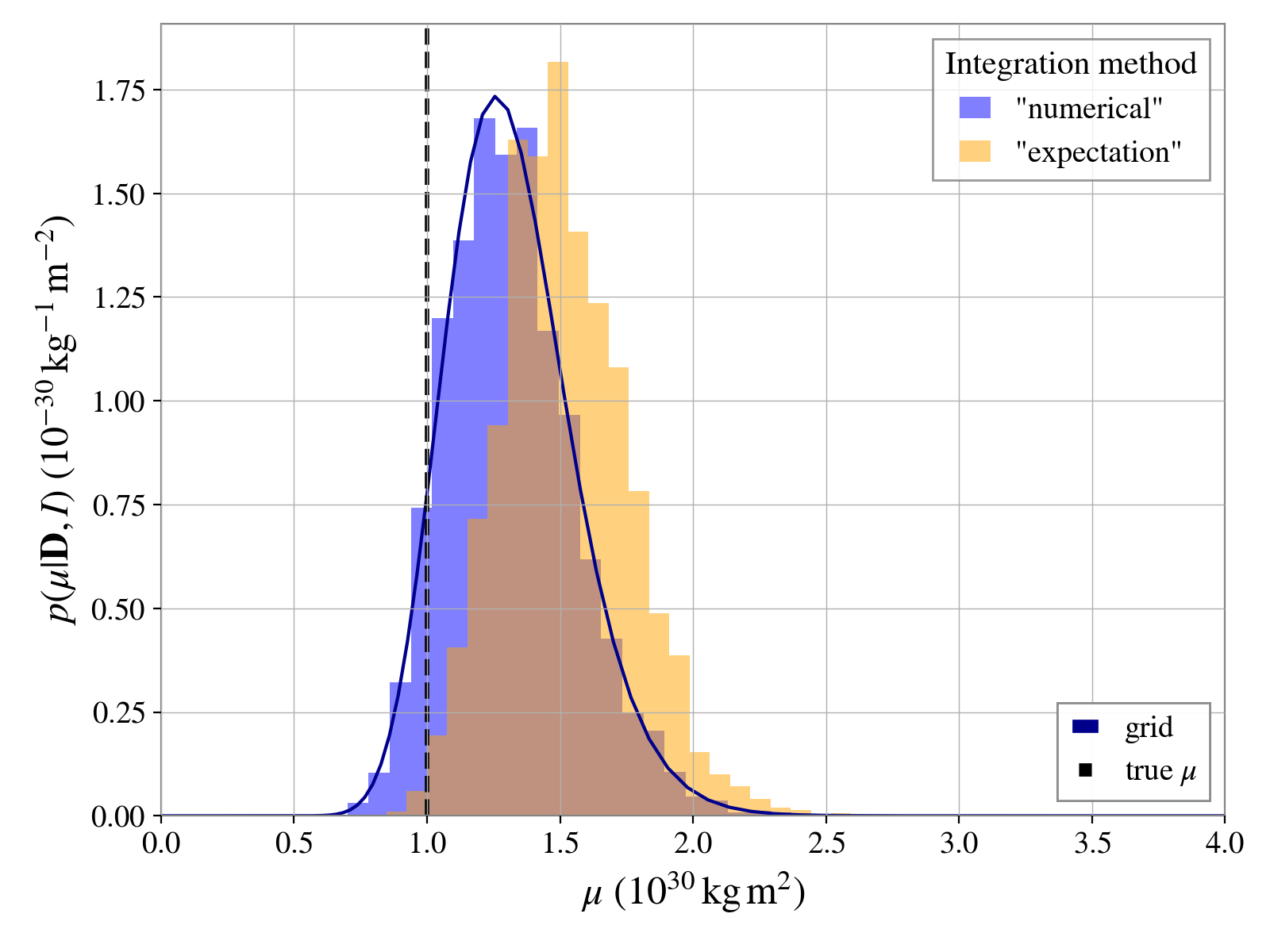
For comparison, we can plot the results from these different methods as below (assuming the Result output of using the “expectation value” method is stored in res2):

from matplotlib import pyplot as plt
from matplotlib import rc

# set fonts
rc("mathtext", **{"fontset": "stix"})
rc("font", **{"family": "STIXGeneral"})

# plot posteriors on the exponential distribution hyperparameter mu
fig, ax = plt.subplots(figsize=(8,6))
scale = 1e30  # scale values so histogram works with density=True argument
truth = 1e30  # the known simulation values of mu
ax.hist(  # posterior using "numerical" method
    res.posterior["mu"] / scale,
    density=True,
    histtype="stepfilled",
    alpha=0.5,
    color="blue",
    bins=25,
    label="\"numerical\"",
)
ax.hist(  # posterior using "expectation value" method
    res2.posterior["mu"] / scale,
    density=True,
    histtype="stepfilled",
    alpha=0.5,
    color="orange",
    bins=25,
    label="\"expectation\"",
)

# over plot the distribution as evaluated on a grid
ax.plot(muvalues / scale, postgrid * scale, "darkblue", label="grid")

# add a line showing the "truth"
ax.axvline(truth / scale, color="k", ls="--", lw=2, label="true $\mu$")

ax.set_xlim([0, 4])
ax.set_xlabel(r"$\mu$ ($10^{30}\,{\rm kg}\,{\rm m}^2$)", fontsize=18);
ax.set_ylabel(r"$p(\mu|\mathbf{D}, I)$ ($10^{-30}\,{\rm kg}^{-1}\,{\rm m}^{-2}$)", fontsize=18);

# set axis label font size
for item in ax.get_xticklabels() + ax.get_yticklabels():
    item.set_fontsize(14)

# add legends
leg1 = plt.legend(
    handles=ax.get_legend_handles_labels()[0][2:],
    title="Integration method",
    fontsize=14,
    title_fontsize=15,
    loc="upper right",
)
leg2 = plt.legend(
    ax.get_lines()[0:2],
    ax.get_legend_handles_labels()[1][0:2],
    loc="lower right",
    fontsize=14,
)
ax.add_artist(leg1)
ax.add_artist(leg2)
fig.tight_layout()
fig.savefig("muposterior.png", dpi=200)

It is interesting to look at the distribution of the signal-to-noise ratios of the simulation versus the recovered maximum a-posteriori signal to noise ratios. Another informative plot is a posterior predictive plot that checks the recovered exponential distribution matches the simulated distribution of \(Q_{22}\) values. Both these are shown below.

from bilby.core.prior import Exponential
from cwinpy import PulsarParameters
import glob
import json
from matplotlib import pyplot as plt
from matplotlib import rc

# true mu value
truth = 1e30
scale = 1e30 # scale values so histogram works with density=True argument

# load in SNRs
snrfiles = glob.glob("/home/user/exponential/results/J*/*snr")
injsnrs = []
recsnrs = []
for sf in snrfiles:
    with open(sf, "r") as fp:
        d = json.load(fp)
    injsnrs.append(d["Injected SNR"])
    recsnrs.append(d["Maximum a-posteriori SNR"])

# load in simulation pulsar parameters and extract Q22 values
pulsarfiles = glob.glob("/home/user/exponential/pulsars/*.par")
trueq22 = np.array([PulsarParameters(pf)["Q22"] for pf in pulsarfiles])

# create plot
rc("mathtext", **{"fontset": "stix"})
rc("font", **{"family": "STIXGeneral"})
rc("font", **{"size": 16})
fig, ax = plt.subplots(1, 2, figsize=(12, 6))

# plot true SNR vs recovered SNR
ax[0].plot(injsnrs, recsnrs, "bo", markersize=10, alpha=0.5)
ax[0].set_xscale("log")
ax[0].set_yscale("log")
ax[0].set_xlabel("Injected SNR", fontsize=16);
ax[0].set_ylabel("Maximum a-posteriori SNR", fontsize=16);

# plot posterior predictive
nsamples = 500  # get 500 samples to use for posterior predictive plot
q22values = np.logspace(28, np.log10(2 * np.max(trueq22)), 10000)

for pdf in mqd.posterior_predictive(q22values, nsamples=nsamples):
    ax[1].plot(q22values / scale, pdf * scale, color="orange", alpha=0.05)
ax[1].plot(  # add "true" distribution
    q22values / scale,
    Exponential(mu=truth / scale, name="mu").prob(q22values / scale),
    color='k',
    lw=2,
    ls="--",
)

# add histogram and rug plot of simulated Q22 values
ax[1].plot(trueq22 / scale, np.zeros_like(trueq22), '|', color='k', ms=15, alpha=0.5)
ax[1].hist(trueq22 / scale, bins=15, histtype="step", density=True)
ax[1].set_xlim([0, q22values.max() / scale])
ax[1].set_xlabel(r"$Q_{22}$ ($10^{30}\,{\rm kg}\,{\rm m}^2$)", fontsize=16)
ax[1].set_ylabel(r"$p(Q_{22}|\mathbf{D}, I)$", fontsize=16)
ax[1].set_title("Posterior predictive check", fontsize=17)

fig.tight_layout()
fig.savefig("muposteriorpredictive.png", dpi=200)

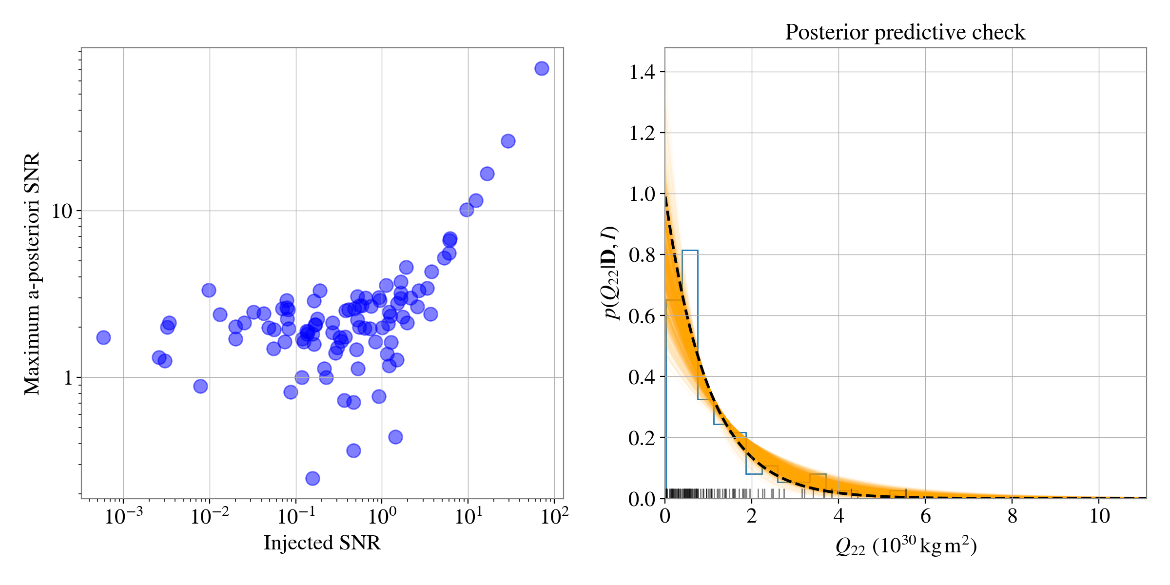
It can be seen that the recovered exponential distributions agree well with the true distribution of \(Q_{22}\) values generated in the simulation.

Model comparison

We can estimate the hyperparameters of a different distribution based on the same simulated pulsar population. From this we can use the calculated marginal likelihoods for the two distributions to compare which distribution fits the data best.

Below, we use chose to try and fit another simple distribution with a single hyperparameter, a BoundedGaussianDistribution distribution. This distribution can be used to fit a mixture model of Gaussians to the data (bounded at zero, so that only positive values are allowed), but here we will just assume a single mode. The peak of the mode will be fixed at zero and the width, \(\sigma\), will be given a HalfNormal prior with the same scale of \(\sigma = 10^{34}\,{\textrm{kg}}\,{\textrm m}^2\) as used for \(\mu\) previously.

Note

Within a BoundedGaussianDistribution the distribution modes will be held as parameters called muX, the widths will be held as parameters called sigmaX, and the mode weights will be held as parameters called weightX, where X will be an index for the mode starting at zero. E.g., for a distribution defined with a single mode, the parameters held will be mu0, sigma0 and weight0.

# set up a Gaussian distribution (bounded at zero) with one mode at zero and
# a width to be fitted using sigma
sigma = 1e34
distkwargs = {
    "mus": [0],  # fix the peak of the single mode at zero
    "sigmas": [HalfNormal(sigma, name="sigma")],  # set prior on width of the mode
    "weights": [1],
}
distribution = "gaussian"  # the keyword to use a bounded Gaussian distribution
sampler_kwargs = {
    "sample": "unif",
    "nlive": 500,
    "gzip": True,
    "outdir": "gaussian_distribution",
    "label": "test",
    "check_point_plot": False,
}
bins = 500
mqdgauss = MassQuadrupoleDistribution(
    data=data,
    distribution=distribution,
    distkwargs=distkwargs,
    bins=bins,
   sampler_kwargs=sampler_kwargs,
)

# sample from the sigma hyperparameters
resgauss = mqdgauss.sample()

We can get the Bayes factor between the two distributions with:

# get the base-10 log Bayes factor between the two models (exponential
# distribution as the numerator and Gaussian as the denominator
bayesfactor = res.log_10_evidence - resgauss.log_10_evidence

In this case the bayesfactor value is -0.75, i.e., the bounded Gaussian distribution is actually favoured over the (true) exponential distribution by a factor of \(10^{0.75} = 5.6\)! A Bayes factor of ~6 is not convincing evidence to favour one model over the other, but it shows that in some cases it can be tricky to distinguish between distributions.

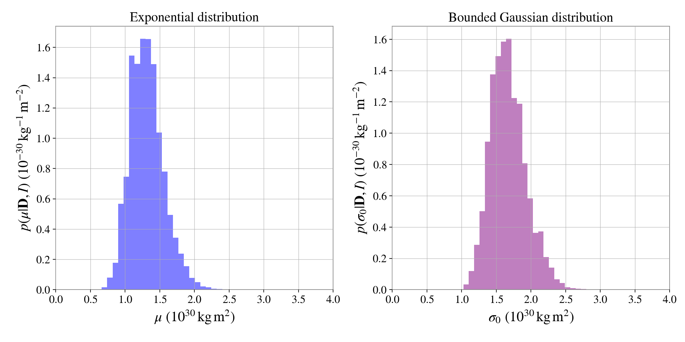
We can plot the posterior distributions for the hyperparameters from the exponential and Gaussian distributions side-by-side:

# plot posteriors on the exponential distribution hyperparameter mu
fig, ax = plt.subplots(1, 2, figsize=(12, 6))
scale = 1e30  # scale values so histogram works with density=True argument

# plot mu from exponential distribution
ax[0].hist(
    res.posterior["mu"] / scale,
    density=True,
    histtype="stepfilled",
    alpha=0.5, color="blue",
    bins=25,
)

# plot sigma from gaussian distribution
ax[1].hist(
    resgauss.posterior["sigma0"] / scale,
    density=True,
    histtype="stepfilled",
    alpha=0.5, color="purple",
    bins=25,
)

ax[0].set_xlim([0, 4])
ax[0].set_xlabel(r"$\mu$ ($10^{30}\,{\rm kg}\,{\rm m}^2$)", fontsize=18)
ax[0].set_ylabel(r"$p(\mu|\mathbf{D}, I)$ ($10^{-30}\,{\rm kg}^{-1}\,{\rm m}^{-2}$)", fontsize=18)
ax[0].set_title("Exponential distribution")

ax[1].set_xlim([0, 4])
ax[1].set_xlabel(r"$\sigma_0$ ($10^{30}\,{\rm kg}\,{\rm m}^2$)", fontsize=18)
ax[1].set_ylabel(r"$p(\sigma_0|\mathbf{D}, I)$ ($10^{-30}\,{\rm kg}^{-1}\,{\rm m}^{-2}$)", fontsize=18)
ax[1].set_title("Bounded Gaussian distribution")

fig.tight_layout()
fig.savefig("musigmaposterior.png", dpi=200)

The trickiness of distinguishing the distributions in this case is highlighted using the posterior predictive plots:

fig, ax = plt.subplots(1, 2, figsize=(12, 6), sharey=True)

# plot posterior predictive for exponential distribution
nsamples = 500  # get 500 samples to use for posterior predictive plot
q22values = np.logspace(28, np.log10(2 * np.max(trueq22)), 10000)

scale = 1e30  # scale values so histogram works with density=True argument
for pdf in mqd.posterior_predictive(q22values, nsamples=nsamples):
    ax[0].plot(q22values / scale, pdf * scale, color="orange", alpha=0.05)
ax[0].plot(  # add "true" distribution
    q22values / scale,
    Exponential(mu=truth / scale, name="mu").prob(q22values / scale),
    color='k',
    lw=2,
    ls="--",
)

# add histogram and rug plot of simulated Q22 values
ax[0].plot(trueq22 / scale, np.zeros_like(trueq22), '|', color='k', ms=15, alpha=0.5)
ax[0].hist(trueq22 / scale, bins=15, histtype="step", density=True)
ax[0].set_xlim([0, q22values.max() / scale])
ax[0].set_xlabel(r"$Q_{22}$ ($10^{30}\,{\rm kg}\,{\rm m}^2$)", fontsize=16)
ax[0].set_ylabel(r"$p(Q_{22}|\mathbf{D}, I)$", fontsize=16)
ax[0].set_title("Exponential distribution", fontsize=17)

# plot posterior predictive for bounded Gaussian distribution
for pdf in mqdgauss.posterior_predictive(q22values, nsamples=nsamples):
    ax[1].plot(q22values / scale, pdf * scale, color="red", alpha=0.05)
ax[1].plot(  # add "true" distribution
    q22values / scale,
    Exponential(mu=truth / scale, name="mu").prob(q22values / scale),
    color='k',
    lw=2,
    ls="--",
)

# add histogram and rug plot of simulated Q22 values
ax[1].plot(trueq22 / scale, np.zeros_like(trueq22), '|', color='k', ms=15, alpha=0.5)
ax[1].hist(trueq22 / scale, bins=15, histtype="step", density=True)
ax[1].set_xlim([0, q22values.max() / scale])
ax[1].set_xlabel(r"$Q_{22}$ ($10^{30}\,{\rm kg}\,{\rm m}^2$)", fontsize=16)
ax[1].set_title("Bounded Gaussian distribution", fontsize=17)

fig.tight_layout()
fig.savefig("musigmaposteriorpredictive.png", dpi=200)

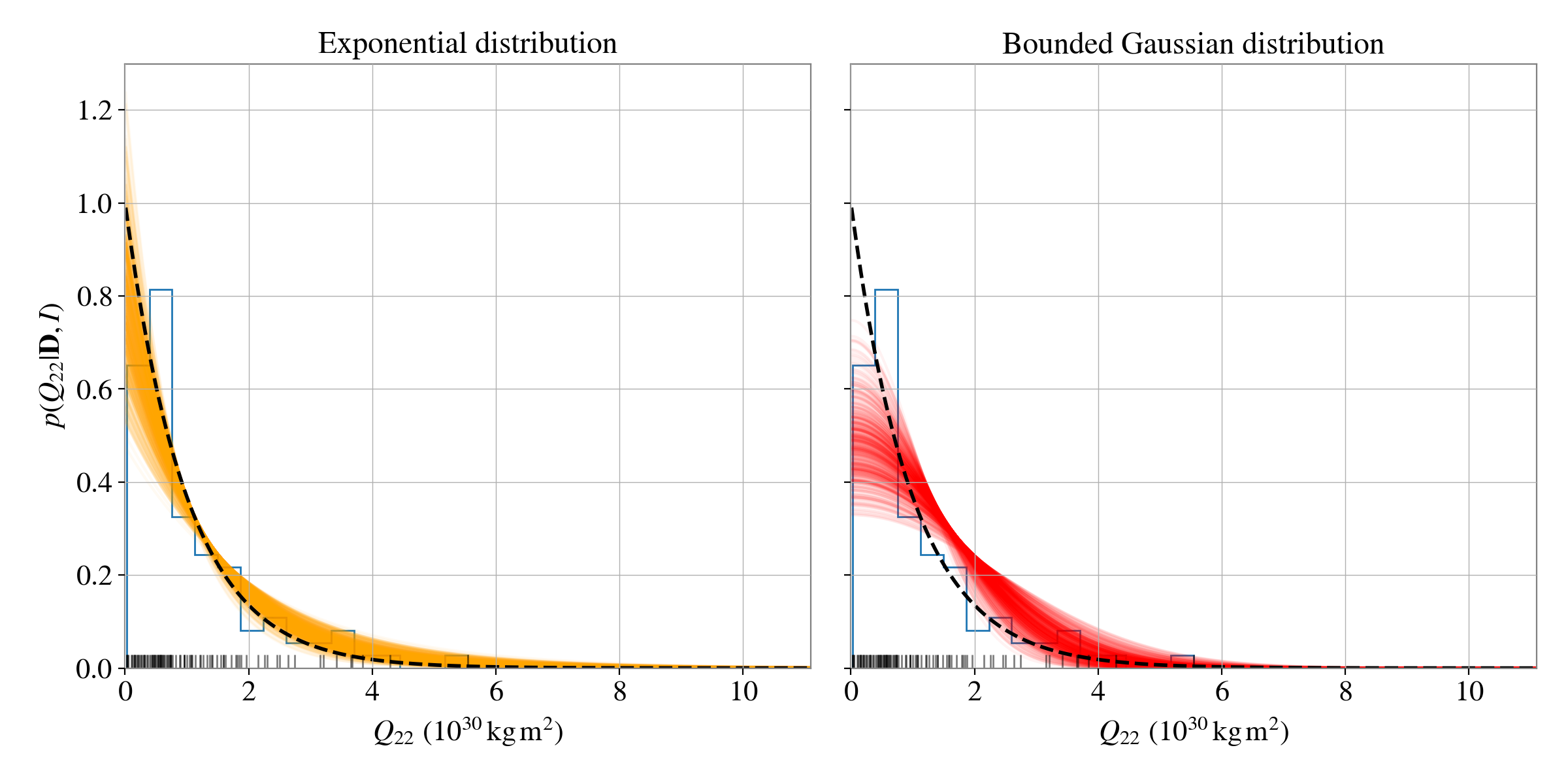
We can see that both models do a reasonable job at recovering the simulated distribution.

Hierarchical module API

Classes for hierarchical parameter inference.

class BaseDistribution(name, disttype, hyperparameters={}, low=-inf, high=inf)

Bases: object

The base class for the distribution, as defined by a set of hyperparameters, that you want to fit.

Parameters:

• name (str) – The parameter for which this distribution is the prior.

• disttype (str) – The type of distribution, e.g., ‘exponential’, ‘gaussian’.

• hyperparameters (dict) – A dictionary of hyperparameters for the distribution with the keys giving the parameter names, and values giving their fixed value, or a bilby.core.prior.Prior for values that are to be inferred.

• low (float) – The lower bound of the distribution

• high (float) – The upper bound of the distribution

property fixed

Return a dictionary keyed to parameter names and with boolean values indicating whether the parameter is fixed (True), or to be inferred (False).

log_pdf(value, hyperparameters)

The natural logarithm of the distribution’s probability density function at the given value.

Parameters:

• value (float) – The value at which to evaluate the probability.

• hyperparameters (dict) – A dictionary of the hyperparameter values that define the current state of the distribution.

Returns:

The natural logarithm of the probability.

Return type:

lnpdf

pdf(value, hyperparameters)

The distribution’s probability density function at the given value.

Parameters:

• value (float) – The value at which to evaluate the probability.

• hyperparameters (dict) – A dictionary of the hyperparameter values that define the current state of the distribution.

Returns:

The probability density.

Return type:

pdf

sample(hyperparameters, size=1)

Draw a sample from the distribution as defined by the given hyperparameters.

Parameters:

• hyperparameters (dict) – A dictionary of the hyperparameter values that define the current state of the distribution.

• size (int) – The number of samples to draw from the distribution.

Returns:

A sample, or set of samples, from the distribution.

Return type:

sample

property unknown_parameters

A list of the parameters that are to be inferred.

property unknown_priors

A list of the Prior for the parameters that are to be inferred.

property unpacked_fixed

Return a flattened version of fixed, with multivalued parameters indexed.

class BoundedGaussianDistribution(name, mus=[], sigmas=[], weights=None, low=0.0, high=inf)

Bases: BaseDistribution

A distribution to define estimating the parameters of a (potentially multi-modal) bounded Gaussian distribution.

An example of using this distribution for a two component Gaussian distribution bounded at zero and with unknown mean, standard deviations and weights would be:

>>> from bilby.core.prior import HalfNormal, LogUniform, DirichletPriorDict
>>> # set priors for means (half-Normal distributions with mode at 0)
>>> mus = [HalfNormal(10.0, name="mu0"), HalfNormal(10.0, name="mu1")]
>>> # set priors for standard deviations (log uniform distributions)
>>> sigmas = [LogUniform(name="sigma0", minimum=0.0001, maximum=100.0),
              LogUniform(name="sigma1", minimum=0.0001, maximum=100.0)]
>>> # set a Dirichlet prior on the weights (i.e., they must add up to 1)
>>> weights = DirichletPriorDict(n_dim=2, label="weight")
>>> dist = BoundedGaussianDistribution("x", mus=mus, sigmas=sigmas, weights=weights)

Note that if using a Dirichlet prior on the weights all weights must be included and none can be set as fixed.

Parameters:

• name (str) – See BaseDistribution

• mus (array_like) – A list of values of the means of each mode of the Gaussian.

• sigmas (array_like) – A list of values of the standard deviations of each mode of the Gaussian.

• weights (array_like) – A list of values of the weights (relative probabilities) of each mode. This will default to equal weights if not given. If wanting to estimate multiple weights a DirichletPriorDict should be used as in the example above.

• low (float) – The lower bound of the distribution (defaults to 0, i.e., only positive values are allowed)

• high (float) – The upper bound of the distribution (default to infinity)

log_pdf(value, hyperparameters={})

The natural logarithm of the pdf of a 1d (potentially multi-modal) Gaussian probability distribution.

Parameters:

• value (float) – The value at which the probability is to be evaluated.

• hyperparameters (dict) – A dictionary containing the current values of the hyperparameters that need to be inferred. If there are multiple modes and weights are not fixed then the hyperparameters should include n-1 weights values, where n is the number of modes.

Returns:

The natural logarithm of the probability density at the given value.

Return type:

logpdf

sample(hyperparameters={}, size=1)

Draw a sample from the bounded Gaussian distribution as defined by the given hyperparameters.

Parameters:

• hyperparameters (dict) – A dictionary of the hyperparameter values that define the current state of the distribution. If there are multiple modes and weights are not fixed then the hyperparameters should include n-1 weights values, where n is the number of modes.

• size (int) – The number of samples to draw. Default is 1.

Returns:

A sample, or set of samples, from the distribution.

Return type:

sample

DISTRIBUTION_REQUIREMENTS = {'deltafunction': ['peak'], 'exponential': ['mu'], 'gaussian': ['mu', 'sigma', 'weight'], 'histogram': ['weight'], 'powerlaw': ['alpha', 'minimum', 'maximum']}

Allowed distributions and their required hyperparameters

class DeltaFunctionDistribution(name, peak)

Bases: BaseDistribution

A distribution defining a delta function (useful if wanting to fix a parameter at a specific value if creating signals, or use as a null model).

Parameters:

• name (str) – See BaseDistribution

• peak (float) – The value at which the delta function is non-zero.

log_pdf(value, hyperparameters={})

The natural logarithm of the pdf of a delta function distribution.

Parameters:

• value (float) – The value at which the probability is to be evaluated.

• hyperparameters (dict) – A dictionary containing the current values of the hyperparameters that need to be inferred.

Returns:

The natural logarithm of the probability at the given value.

Return type:

logpdf

sample(hyperparameters={}, size=1)

Return the position of the delta function.

Parameters:

• hyperparameters (dict) – A dictionary of the hyperparameter values (peak) that define the current state of the distribution.

• size (int) – The number of samples to draw from the distribution.

Returns:

A sample, or set of samples, from the distribution.

Return type:

sample

class ExponentialDistribution(name, mu)

Bases: BaseDistribution

A distribution to define estimating the parameters of an exponential distribution.

Parameters:

• name (str) – See BaseDistribution

• mu (float, Prior) – The mean of the exponential distribution.

log_pdf(value, hyperparameters={})

The natural logarithm of the pdf of an exponential distribution.

Parameters:

• value (float) – The value at which the probability is to be evaluated.

• hyperparameters (dict) – A dictionary containing the current values of the hyperparameters that need to be inferred.

Returns:

The natural logarithm of the probability at the given value.

Return type:

logpdf

sample(hyperparameters={}, size=1)

Draw a sample from the exponential distribution as defined by the given hyperparameters.

Parameters:

• hyperparameters (dict) – A dictionary of the hyperparameter values (mu) that define the current state of the distribution.

• size (int) – The number of samples to draw from the distribution.

Returns:

A sample, or set of samples, from the distribution.

Return type:

sample

class HistogramDistribution(name, low, high, nbins=10)

Bases: BaseDistribution

A distribution to define estimating the bin weights of a non-parameteric histogram-type distribution. The priors for the bin weights will be a Dirichlet prior.

An example of using this distribution for a 10 bin histogram would be:

>>> # set the number of bins and bounds
>>> nbins = 20
>>> lowerbound = 0.0
>>> upperbound = 10.0
>>> dist = HistogramDistribution("x", low=lowerbound, high=upperbound, nbins=nbins)

Parameters:

• name (str) – See BaseDistribution

• low (float) – The lower bound of the distribution (required).

• high (float) – The upper bound of the distribution (required).

• nbins (int) – An integer number of histogram bins to use (defaults to 10).

log_pdf(value, hyperparameters={})

The natural logarithm of the pdf of a histogrammed distribution.

Parameters:

• value (float) – The value at which the probability is to be evaluated.

• hyperparameters (dict) – A dictionary containing the current values of the hyperparameters that need to be inferred. For a histogram with n bins, the hyperparameters should include n-1 weights values.

Returns:

The natural logarithm of the probability density at the given value.

Return type:

logpdf

sample(hyperparameters={}, size=1)

Draw a sample from the histogram distribution as defined by the given hyperparameters.

Parameters:

• hyperparameters (dict) – A dictionary of the hyperparameter values that define the current state of the distribution. If there are n bins in the histogram, then the hyperparameters should include n-1 weights values.

• size (int) – The number of samples to draw. Default is 1.

Returns:

A sample, or set of samples, from the distribution.

Return type:

sample

class MassQuadrupoleDistribution(data=None, gridrange=None, bins=100, gridtype=None, distribution=None, distkwargs=None, bw='scott', sampler='dynesty', sampler_kwargs={}, grid=None, integration_method='numerical', nsamples=None, use_ellipticity=False)

Bases: object

A class to infer the hyperparameters of the \(l=m=2\) mass quadrupole distribution (or fiducial ellipticity \(\varepsilon\)) for a given selection of known pulsars (see, for example, [2]).

The class currently can attempt to fit the hyperparameters for the following distributions:

• a \(n\)-mode bounded Gaussian distribution defined by either fixed or unknown means, standard deviations and weights;

• an exponential distribution defined by an unknown mean.

• a power law distribution defined by an unknown power law index and fixed or unknown bounds.

All distributions do not allow the quadrupole value to become negative.

Parameters:

• data (bilby.core.result.ResultList) – A bilby.core.result.ResultList of outputs from running source parameter estimation using bilby for a set of individual CW sources. These can be from MCMC or nested sampler runs, but only the latter can be used if requiring a properly normalised evidence value.

• gridrange (array_like) – A list of values at which the \(Q_{22}\) parameter posteriors should be interpolated, or a lower and upper bound in the range of values, which will be split into bins points spaced linearly in log-space (unless gridtype'' is set to a value other than ``"log"). If not supplied this will instead be set using the posterior samples, with a minimum value at zero and a maximum given by the maximum of all posterior samples.

• bins (int) – The number of bins at which the posterior will be interpolated.

• gridtype (str) – This sets the grid bin spacing used for assigning the interpolation grid. It defaults to spacings that are uniform in log-space for distributions other than cwinpy.hierarchical.HistogramDistribution for which case the spacing defaults to linear. Values can either be "log" or "linear" to force one or other spacing.

• distribution (cwinpy.hierarchical.BaseDistribution, str) – A predefined distribution, or string giving a valid distribution name. This is the distribution for which the hyperparameters are going to be inferred. If using a string, the distribution keyword arguments must be passed using distkwargs.

• distkwargs (dict) – A dictionary of keyword arguments for the distribution that is being inferred.

• bw (str, scalar, callable) – See the bw_method argument for scipy.stats.gaussian_kde.

• sampler (str) – The name of the stochastic sampler method used by bilby for sampling the posterior. This defaults to use ‘dynesty’.

• sampler_kwargs (dict) – A dictionary of arguments required by the given sampler.

• grid (dict) – A dictionary of values that define a grid in the parameter and hyperparameter space that can be used by a bilby.core.grid.Grid. If given sampling will be performed on the grid, rather than using the stochastic sampler.

• integration_method (str) – The method to use for integration over the \(Q_{22}\) parameter for each source. Default is ‘numerical’ to perform trapezium rule integration. Other allowed values are: ‘sample’ to sample over each individual \(Q_{22}\) parameter for each source; or, ‘expectation’, which uses the \(Q_{22}\) posterior samples to approximate the expectation value of the hyperparameter distribution. At the moment, these two additional methods may not be correct/reliable.

• nsamples (int) – This sets the number of posterior samples to store for either estimating KDEs or calculating expectation values from those passed in the data. This allows downsampling of large numbers of samples by randomly drawing a subsection of samples. If the number given is larger than the total number of samples for a given pulsar, then all samples will be used in that case. The default will be to use all samples, but this may lead to memory issues when using large numbers of pulsars.

• use_ellipticity (bool) – If True, work with fiducial ellipticity \(\varepsilon\) rather than mass quadrupole.

add_data(data, bw='scott', nsamples=None)

Set the data, i.e., the individual source posterior distributions, on which the hierarchical analysis will be performed.

The posterior samples must include the Q22 \(l=m=2\) parameter, or the fiducial ellipticity parameter ELL, for this inference to be performed.

If using the “numerical” integration method, upon running the sample() method, these samples will be converted to a KDE (reflected about zero to avoid edge effects, and re-normalised, although the bandwidth will be calculated using the unreflected samples), using scipy.stats.gaussian_kde, which will be used as the data for hierarchical inference. If the posterior samples come with a Bayesian evidence value, and the prior is present, then these are used to convert the posterior distribution into a likelihood, which is what is then stored in the interpolation function.

If using the “expectation” integration method, and if the posterior samples were not estimated using a uniform prior on Q22/ELL, then the samples will be resampled from a uniform prior to attempt to generate samples from the likelihood.

Parameters:

• data (bilby.core.result.ResultList) – A list, or single, results from bilby containing posterior samples for a set of sources, or individual source.

• bw (str, scale, callable) – The Gaussian KDE bandwidth calculation method as required by scipy.stats.gaussian_kde. The default is the ‘scott’ method.

• nsamples (int) – This sets the number of posterior samples to store and use from those passed in the data. This allows downsampling of large numbers of samples by randomly drawing a subsection of samples. If the number given is larger than the total number of samples for a given pulsar, then all samples will be used in that case. The default will be to use all samples, but this may lead to memory issues when using large numbers of pulsars.

property interpolated_log_kdes

Return the list of interpolation functions for the natural logarithm of the \(Q_{22}\) likelihood functions after a Gaussian KDE has been applied.

posterior_predictive(points, nsamples=100)

Return an iterator that will draw samples from the distribution hyperparameter posterior (once sample() has been run) and returns the associated distribution evaluated at a set of points.

Currently this is only implemented to work using samples from a stochastic sampling method rather than posteriors evaluated on a grid.

Parameters:

• points (array_like) – An array of Q22/ellipticity values at which to evaluate the distribution.

• nsamples (int) – The number of samples to draw from the distribution. This defaults to 100, but must be less than the number of posterior samples.

property result

Return the bilby object containing the results. If evaluating the posterior over a grid this is a bilby.core.grid.Grid object. If sampling using a stochastic sampler, this is a bilby.core.result.Result object. If sampling has not yet been performed this returns None.

sample(**run_kwargs)

Sample the posterior distribution using bilby. This can take keyword arguments required by the bilby run_sampler() function.

set_distribution(distribution, distkwargs={})

Set the distribution who’s hyperparameters are going to be inferred.

Parameters:

• distribution (cwinpy.hierarchical.BaseDistribution, str) – A predefined distribution, or string giving a valid distribution name. If using a string, the distribution keyword arguments must be passed using distkwargs.

• distkwargs (dict) – A dictionary of keyword arguments for the distribution that is being inferred.

set_grid(grid)

Set a grid on which to evaluate the hyperparameter posterior, as used by bilby.core.grid.Grid.

Parameters:

grid (dict) – A dictionary of values that define a grid in the hyperparameter space that can be used by a bilby.core.grid.Grid class.

set_integration_method(integration_method='numerical')

Set the method to use for integration over the \(Q_{22}\) parameter for each source.

Parameters:

integration_method (str) – Default is ‘numerical’ to perform trapezium rule integration. The other allowed value is ‘expectation’, which uses the \(Q_{22}\) posterior samples to approximate the expectation value of the hyperparameter distribution.

set_range(gridrange, bins=100, gridtype=None)

Set the values of \(Q_{22}\), or ellipticity \(\varepsilon\), either directly, or as a set of points linear in log-space defined by a lower and upper bounds and number of bins, at which to evaluate the posterior samples via their KDE to make an interpolator.

Parameters:

• gridrange (array_like) – If this array contains two values it is assumed that these are the lower and upper bounds of a range, and the bins parameter sets the number of bins in log-space that the range will be split into. Otherwise, if more than two values are given it is assumed these are the values for \(Q_{22}\) or \(\varepsilon\).

• bins (int) – The number of bins the range is split into.

• gridtype (str) – Set whether to have grid-spacing be "linear" or linear in log-10 space ("log"). By default, for distribution’s other than cwinpy.hierarchical.HistogramDistribution the default will be linear in log-10 space.

set_sampler(sampler='dynesty', sampler_kwargs={})

Set the stochastic sampling method for bilby to use when sampling the parameter and hyperparameter posteriors.

Parameters:

• sampler (str) – The name of the stochastic sampler method used by bilby for sampling the posterior. This defaults to use ‘dynesty’.

• sampler_kwargs (dict) – A dictionary of arguments required by the given sampler.

class MassQuadrupoleDistributionLikelihood(distribution, likelihoods=None, grid=None, samples=None)

Bases: Likelihood

The likelihood function for the inferring the hyperparameters of the mass quadrupole, \(Q_{22}\), distribution (or equivalently the fiducial ellipticity distribution).

Parameters:

• distribution (cwinpy.hierarchical.BaseDistribution) – The probability distribution for which the hyperparameters are going to be inferred.

• likelihoods (list) – A list of interpolation functions each of which gives the likelihood function for a single source.

• grid (array_like) – If given, the integration over the mass quadrupole distribution for each source is performed numerically on at these grid points. If not given, individual samples from \(Q_{22}\) will be drawn from each source (i.e., equivalent to having a new \(Q_{22}\) parameter for each source in the sampler).

• samples (list) – A list of arrays of \(Q_{22}\) samples for each source. If this is given then these samples will be used to approximate the integral over independent \(Q_{22}\) variables for each source.

Empty likelihood class to be subclassed by other likelihoods

Parameters:

parameters (dict) – A dictionary of the parameter names and associated values

log_likelihood()

Evaluate the log likelihood.

noise_log_likelihood()

The log-likelihood for the unknown hyperparameters being equal to with zero.

Note

For distributions with hyperparameter priors that exclude zero this will always given \(-\infty\).

class PowerLawDistribution(name, alpha, minimum, maximum)

Bases: BaseDistribution

A distribution to define estimating the parameters of a power law distribution.

Parameters:

• name (str) – See BaseDistribution

• alpha (float, Prior) – The power law index of the distribution.

• minimum (float) – A positive finite value giving the lower cutoff of the distribution.

• maximum (float) – A positive finite value giving the upper cutoff of the distribution.

log_pdf(value, hyperparameters={})

The natural logarithm of the pdf of a power law distribution.

Parameters:

• value (float) – The value at which the probability is to be evaluated.

• hyperparameters (dict) – A dictionary containing the current values of the hyperparameters that need to be inferred.

Returns:

The natural logarithm of the probability at the given value.

Return type:

logpdf

sample(hyperparameters={}, size=1)

Draw a sample from the exponential distribution as defined by the given hyperparameters.

Parameters:

• hyperparameters (dict) – A dictionary of the hyperparameter values (alpha, minimum and maximum) that define the current state of the distribution.

• size (int) – The number of samples to draw from the distribution.

Returns:

A sample, or set of samples, from the distribution.

Return type:

sample

create_distribution(name, distribution, distkwargs={})

Function to create a distribution.

An example of creating an exponential distribution, with a half-Gaussian prior on the mean would be:

>>> from bilby.core.prior import HalfGaussian
>>> sigma = 1e34  # width of half-Gaussian prior on mu
>>> distkwargs = {"mu": HalfGaussian(name="mu", sigma=sigma)}
>>> expdist = create_distribution("q22", "exponential", distkwargs)

An example of creating a bimodal-Gaussian distribution, with modes fixed at particular values, fixed weights, but log-uniform priors on the mode widths, would be:

>>> from bilby.core.prior import LogUniform
>>> min = 1e28  # minimum of the width prior
>>> max = 1e38  # maximum of the width prior
>>> modes = [0.0, 1e32]  # fixed modes
>>> weights = [0.7, 0.3]  # fixed weights
>>> sigmas = [
>>>     LogUniform(name="sigma0", minimum=min, maximum=max),
>>>     LogUniform(name="sigma1", minimum=min, maximum=max),
>>> ]
>>> distkwargs = {
>>>     "mu": modes,  # set "mu" for the modes
>>>     "sigma": sigmas,  # set "sigma" for the widths
>>>     "weight": weights,  # set "weight" for the weights
>>> }
>>> gaussdist = create_distribution("q22", "gaussian", distkwargs)

Parameters:

• name (str) – The name of the parameter which the distribution represents.

• distribution (str, cwinpy.hierarchical.BaseDistribution) – A string giving a valid distribution name. This is the distribution for which the hyperparameters are going to be inferred. If using a string, the distribution keyword arguments must be passed using distkwargs.

• distkwargs (dict) – A dictionary of keyword arguments for the distribution that is being inferred.

Returns:

The distribution class.

Return type:

distribution

Hierarchical analysis references

[1] (1,2)

N. K. Johnson-McDaniel & B. J. Owen, PRD, 88, 044004 (2013).

[2] (1,2,3)

M. Pitkin, C. Messenger & X. Fan, PRD, 98, 063001 (2018).

[3]

D. W. Hogg, A. D. Myers & J. Bovy, ApJ, 725, 2166-2175 (2010).